Holonomy, Gyroscopes, and Curvature Measurement

Parallel transport provides a route-dependent comparison between vectors at separated events. If a tetrad is transported around a sufficiently small closed loop and returns rotated or boosted relative to its initial orientation, the leading mismatch is the Riemann tensor contracted with the loop’s oriented area. Reversing the loop reverses the mismatch, giving an immediate sign and systematic-error check.

Required background. We use Riemann curvature and parallel transport and the measurement limits established by the equivalence principles.

Helpful background. The construction is clearest with Minkowski-space transformations, smooth tensor calculus, tetrads and anholonomy, and geodesic transport.

Infinitesimal-loop holonomy

At an event $p$, let two small tangent displacements span an oriented parallelogram. Encode its area by the antisymmetric bivector

$$\Sigma^{\alpha\beta} =\delta a\,\delta b \left(B^\alpha A^\beta-B^\beta A^\alpha\right),$$

where the positive traversal goes first along $\delta a\,A$, then $\delta b\,B$, then back along the opposite sides. Parallel transport a vector $V^\mu$ around the four sides. Let $L$ be a common linear scale: the side displacements $\delta a\,A$ and $\delta b\,B$ have magnitude $O(L)$, and the expansion below takes $L\to0$ at fixed loop shape. With

$$[\nabla_\alpha,\nabla_\beta]V^\mu =R^\mu{}_{\nu\alpha\beta}V^\nu,$$

the returned vector differs by

$$\Delta V^\mu =\frac12R^\mu{}_{\nu\alpha\beta}(p) V^\nu\Sigma^{\alpha\beta} +O(L^3).$$

Carroll motivates this expression from the loop geometry and states the corresponding ordered-side convention explicitly Carroll 1997, § 3, pp. 74–75, Eq. (3.63), PDF. Because different texts reverse either the loop or Riemann convention, a usable measurement protocol must declare both.

The change is linear in area, not perimeter. Connection effects accumulated on individual sides are of order $L$, but coordinate-dependent contributions cancel upon closing the loop. The invariant residue begins at order $RL^2$. The remainder denotes a small-loop Taylor expansion: cubic terms involve $\nabla R$, while quartic terms can involve both $\nabla\nabla R$ and $R^2$. Dropping the cubic term at an event where $\nabla R=0$ does not generally leave only $R^2$ corrections.

Derivation from noncommuting derivatives

Let $A$ and $B$ extend locally to commuting coordinate directions. Compare transporting first along $A$ then $B$ with the reverse order. Expanding both procedures to second order gives

$$\left(\nabla_B\nabla_A-\nabla_A\nabla_B\right)V^\mu =B^\alpha A^\beta R^\mu{}_{\nu\alpha\beta}V^\nu$$

for the stated orientation. Multiplying by $\delta a\,\delta b$ yields the loop formula. If the vector fields do not commute, an additional $\nabla_{[B,A]}V$ term accounts for the failure of their coordinate parallelogram to close; that is a property of the chosen directions, not extra curvature.

Reversing the path sends $\Sigma^{\alpha\beta}$ to $-\Sigma^{\alpha\beta}$ and hence $\Delta V^\mu$ to $-\Delta V^\mu$ at leading order. Traversing the loop twice doubles the leading change only while $|R|L^2\ll1$; finite holonomies compose noncommutatively and need not add linearly.

Constant-curvature check

In a spacetime of constant sectional curvature $K$,

$$R^\mu{}_{\nu\alpha\beta} =K\left(\delta^\mu_\alpha g_{\nu\beta} -\delta^\mu_\beta g_{\nu\alpha}\right).$$

Substitution gives

$$\Delta V^\mu=K\Sigma^\mu{}_{\nu}V^\nu+O(K^2L^4).$$

Here the loop is shrunk homothetically, with fixed shape, in a region of constant $K$. The general cubic correction proportional to $\nabla R$ vanishes because $\nabla R=0$; the next term comes from composing curvature effects and scales as $K^2L^4$. The area bivector generates a rotation for a spacelike loop plane and a boost for a timelike–spacelike plane. The result has the right dimensions: $K$ has units $L^{-2}$, area has units $L^2$, and the holonomy parameter is dimensionless. It vanishes as $K\to0$ and reverses sign with the loop orientation.

This example also checks topology. A sufficiently small contractible loop in flat spacetime has zero holonomy to this order. A large loop on a flat but globally identified space can have nontrivial global holonomy; that does not represent nonzero local Riemann curvature.

Gyroscopes and transported frames

An ideal torque-free gyroscope in geodesic motion carries a parallel-transported spin vector. A physical comparison uses two future-directed carrier paths $\gamma_A$ and $\gamma_B$ from the same preparation event $P$ to a reunion event $Q$. Both carriers move forward in time. The mathematical closed curve follows $\gamma_A$ and the inverse of $\gamma_B$; it does not require a carrier to travel backward in time or around a closed timelike curve in the local laboratory.

Let $U_A,U_B:T_PM\to T_QM$ be the two parallel-transport maps. At reunion, compare both transported vectors in one calibrated tetrad at $Q$. Pulling this comparison back to $P$ gives the holonomy map $U_B^{-1}U_A:T_PM\to T_PM$. The inverse map is a comparison operation, not a second physical trip. Two distinct timelike geodesics cannot generally join the same pair of events inside a convex normal neighborhood, so a small reunion experiment needs controlled accelerations, transfers between observers, or an equivalent network of comparisons.

The experiment is delicate. A torque-free gyroscope on an accelerated path follows Fermi–Walker transport rather than parallel transport. Its acceleration history, changes of carrier, and the final tetrad alignment must therefore be measured and accounted for before identifying the residual with geometric holonomy. Finite loop size samples curvature gradients, and comparing readings at different events requires an additional transport choice. Comparing opposite mathematical loop orientations reverses the leading curvature term; experimentally reversing a protocol cancels an apparatus offset only when that offset is unchanged by the reversal.

Varying the initial vector and the loop plane probes the linear maps $R(A,B)$. Enough independent planes and tetrad directions reconstruct the Riemann tensor subject to its algebraic symmetries. A single loop yields only one curvature-weighted Lorentz transformation.

The figure separates the physical journeys from the algebraic comparison. Follow both arrows upward to the reunion event; only the map in the lower panel uses inverse transport.

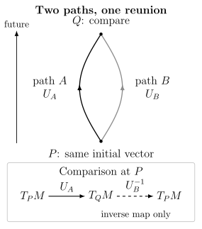
Both carriers travel from $P$ to $Q$, where their transported vectors are compared in one tetrad. The closed-loop map at $P$ is $U_B^{-1}U_A$; the inverse map is not a physical return journey. Gyroscope acceleration and frame alignment must be accounted for before the comparison isolates curvature holonomy. Spacetime schematic, not to scale; no curvature magnitude or rotation angle is implied.

Exercises

For the constant-curvature result, show that reversing $A$ and $B$ reverses the leading holonomy but leaves its magnitude unchanged.

Solution

Interchanging $A$ and $B$ sends

$$\Sigma^{\alpha\beta} \mapsto\delta a\,\delta b (A^\alpha B^\beta-A^\beta B^\alpha) =-\Sigma^{\alpha\beta}.$$

Therefore $\Delta V^\mu=K\Sigma^\mu{}_{\nu}V^\nu$ changes sign. Norms built quadratically from the infinitesimal change are unchanged to their leading nonzero order, as expected for traversing the same geometric loop in the opposite direction.

References

• Carroll, Sean M. “Lecture Notes on General Relativity.” NSF-ITP/97-147, arXiv:gr-qc/9712019v1 (1997). arXiv.