Domains of Dependence

An initial set can determine an event only when every causal history reaching that event is forced to pass through the set. The domain of dependence makes this idea geometric: it identifies the region shielded from causal influence entering around the proposed data surface. It does not, by itself, prove that any particular field equation is well posed. Rather, it supplies the causal region on which a hyperbolic evolution theorem can turn initial data into a unique solution.

Required background. Geodesics and Jacobi Fields supplies inextendible causal curves and their parametrizations. Helpful background. Lorentzian Metrics and Causal Cones fixes the cone convention; Causality and Global Structure places dependence in the causal hierarchy; Partial Differential Equations and Green Functions explains how geometric propagation becomes an initial-value problem.

The future and past dependence sets

Let $(M,g)$ be a time-oriented spacetime without boundary, and let $S\subset M$ be achronal: no two points of $S$ can be joined by a timelike curve. The future domain of dependence of $S$ is

$$D^+(S)=\left\{p\in M:\text{ every past-inextendible causal curve through }p \text{ meets }S\right\}.$$

The past domain $D^-(S)$ is defined by reversing past and future, and

$$D(S)=D^+(S)\cup D^-(S).$$

Here “inextendible” means inextendible as a causal curve in the spacetime under consideration. It is not enough to examine causal curves that are convenient, geodesic, or complete. An accelerated timelike curve and a null curve that approaches a missing point are equally legitimate tests. This universal quantifier is the substance of the definition.

The time direction is easy to check. To decide whether $p\in D^+(S)$, trace past-inextendible curves from $p$: data on $S$ could influence $p$ only from the past. To decide whether $p\in D^-(S)$, trace future-inextendible curves. Points of $S$ belong to both sets under the usual convention that a curve through such a point meets $S$ there.

Achronality prevents timelike return to $S$, but it need not prevent a causal curve from lying along a null segment of $S$. Thus a general achronal Cauchy hypersurface may be met by a causal curve in a segment rather than at exactly one point. A spacelike or acausal data surface removes that ambiguity. The definition and these distinctions are stated precisely in Minguzzi and Sánchez 2008, §3.11.2, pp. 43–44.

What dependence does—and does not—say

The condition $p\in D^+(S)$ says that no past-directed causal history from $p$ can avoid $S$. Equivalently, there is no causal channel by which information relevant at $p$ can enter the spacetime from a missing region, a naked edge, or an unprescribed boundary without first crossing $S$. This is why $D^+(S)$ is the natural maximal candidate region for prediction from data on $S$.

That interpretation has two qualifications. First, causal geometry supplies only a necessary stage of determinism. A specified system of equations must also have existence, uniqueness, and continuous dependence for the chosen data. A badly posed equation is not rescued by a globally good causal geometry. Second, dependence is relative to $S$. Enlarging the set can enlarge the region:

$$S_1\subset S_2 \quad\Longrightarrow\quad D^\pm(S_1)\subset D^\pm(S_2),$$

because every curve that meets $S_1$ also meets $S_2$. The converse implication need not hold, and the domain is not determined by the local geometry of $S$ alone.

Nor is $D^+(S)$ merely $J^+(S)$. Membership in $J^+(S)$ asks whether some future-directed causal curve begins on $S$ and reaches $p$. Membership in $D^+(S)$ controls every past-inextendible causal curve through $p$. Existence and universal interception are different logical statements. This difference is the bridge from the causal relations of the preceding chapter to global prediction.

A diamond in Minkowski spacetime

In two-dimensional Minkowski spacetime with

$$ds^2=-dt^2+dx^2,$$

take the closed interval

$$S=\{(0,x):-a\leq x\leq a\},\qquad a>0.$$

For a point $p=(t,x)$ with $t>0$, the two past-directed null rays meet the line $t=0$ at $x-t$ and $x+t$. Every past-directed causal curve from $p$ meets $S$ exactly when both null endpoints lie in the interval. Therefore

$$D^+(S)=S\cup\{(t,x):t>0,\ \lvert x\rvert+t\leq a\}.$$

The result is the closed upper causal diamond based on $S$. A point with $\lvert x\rvert+t>a$ admits a past-directed null ray that passes around an endpoint of $S$, so it is not determined by data on the interval. The null sides are limiting predictability boundaries; their generator structure is developed on Cauchy Horizons and Their Generators.

The figure makes the universal quantifier visible. At $p$, inspect the two limiting past-null rays: every past-directed causal curve lies between them and therefore meets $S$. At $q$, one dashed null ray already avoids $S$, which is enough to fail the definition. The arrows on the sloping sides orient the future Cauchy-horizon generators.

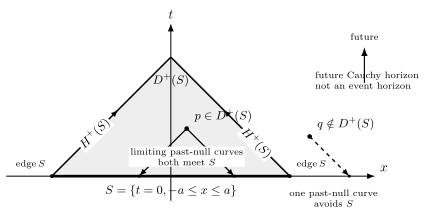
For $S=\{(0,x):-a\leq x\leq a\}$ in $1+1$ Minkowski spacetime, the shaded region is $D^+(S)$. At the interior point $p$, every past-inextendible causal curve through $p$ meets $S$; at $q$, one past-inextendible null curve avoids $S$, which is enough to exclude $q$. The two future-directed null sides form $H^+(S)$, a Cauchy horizon rather than an event horizon. Exact causal incidence for the displayed model; schematic and without physical scale.

If instead $S$ is the entire line $t=0$, every inextendible causal curve in Minkowski spacetime crosses it and $D(S)=M$. This simple check anticipates the definition of a Cauchy Surface. It also illustrates why compactness of $S$ is not required: an entire noncompact hypersurface can be a complete data surface.

Edges, holes, and timelike boundaries

The endpoints of the finite interval are its edge. Near an edge, causal curves can slip from one side of the set to the other without meeting it. Edgelessness is therefore important when an achronal set is intended to behave as a hypersurface rather than as a finite patch of data. A closed achronal set satisfies a useful boundary relation: the boundary of $D^+(S)$ consists of $S$ together with its future Cauchy horizon, with the precise set-theoretic statement given in Minguzzi and Sánchez 2008, Definition 3.73 and the following remarks, pp. 43–44.

Deleting a point exposes a different failure. Start with Minkowski spacetime and remove a point $q$ above $S$. A point $p$ to the future of $q$ can have a past-inextendible causal curve that approaches the missing point and ends there in the punctured manifold. That curve never reaches $S$, so $p$ can leave $D^+(S)$ even though the metric is flat everywhere it is defined. Domains of dependence detect global holes that curvature cannot.

A timelike boundary creates the same logical issue in a controlled form. A past-directed curve may reach the boundary instead of $S$. Data on $S$ alone then do not determine what enters through that boundary; one needs an initial–boundary-value formulation and admissible boundary conditions. The ordinary boundaryless definition should not be stretched into a theorem about anti-de Sitter spacetime, reflecting walls, or finite numerical domains. The precise field-theory distinction is made on Why Global Hyperbolicity Matters for Field Propagation.

Exercise

In two-dimensional Minkowski spacetime, let $S_b=\{(0,x):-b\leq x\leq b\}$ with $0<b<a$. Show directly that $D^+(S_b)\subset D^+(S_a)$, and determine the part of $D^+(S_a)$ not contained in $D^+(S_b)$.

Solution

The null-ray test gives

$$D^+(S_c)=S_c\cup\{(t,x):t>0,\ \lvert x\rvert+t\leq c\}$$

for either $c=a$ or $c=b$. Since $b<a$, the inequality $\lvert x\rvert+t\leq b$ implies $\lvert x\rvert+t\leq a$, and $S_b\subset S_a$; hence the stated inclusion follows. The difference consists of the initial segments $S_a\setminus S_b$ together with the shell

$$\{(t,x):t>0,\ b<\lvert x\rvert+t\leq a\}.$$

The calculation verifies monotonicity but also shows that it is generally strict: adding data near the edge determines an additional causal layer.

References

• Minguzzi, Ettore, “Lorentzian Causality Theory”, Living Reviews in Relativity 22, article 3, §§3–4, 2019.
• Minguzzi, Ettore, and Miguel Sánchez, “The Causal Hierarchy of Spacetimes”, in Recent Developments in Pseudo-Riemannian Geometry, §3.11.2, pp. 43–45 in the arXiv version, European Mathematical Society, 2008.