Event Horizons as Global Boundaries

A future event horizon is the boundary between events that can influence a specified future infinity and events that cannot. This sentence becomes a definition only after the asymptotic end and its conformal completion have been fixed. Because escape is a statement about the entire future, the horizon is teleological: two developments that agree on a large finite region can assign different horizon membership to events in that region. No local curvature measurement can replace the global causal test.

Required background. We use timelike congruences and spatial projection to separate local observer families from asymptotic escape, and hypersurface normals and tangential projectors to interpret smooth horizon portions.

Helpful background. Pseudo-Riemannian metrics and signature supply causal cones, affine and variational geodesics supply null generators, Causality and Global Structure gives the volume-wide map, and Exact Solutions of Einstein’s Equations provides collapse and eternal-solution comparisons.

The black-hole region relative to future infinity

Let $(\widetilde M,\widetilde g)$ be an asymptotically flat physical spacetime admitting an unphysical completion $(M,g,\Omega)$ with

$$g=\Omega^2\widetilde g, \qquad \Omega=0, \qquad d\Omega\ne0$$

on a regular component $\mathscr I^+$ of future null infinity. Causal curves to $\mathscr I^+$ are understood in the completed spacetime, while the regions below contain only physical events. Define the escape region, black-hole region, and future event horizon by

$$\begin{aligned} \mathcal E(\mathscr I^+) &=J^-(\mathscr I^+;M)\cap\widetilde M,\\ \mathcal B(\mathscr I^+) &=\widetilde M\setminus\mathcal E(\mathscr I^+),\\ \mathcal H^+(\mathscr I^+) &=\partial_{\widetilde M}\mathcal B(\mathscr I^+). \end{aligned}$$

Thus $p\in\mathcal B$ means that no future-directed causal curve from $p$ reaches the chosen $\mathscr I^+$. The boundary is taken in the physical spacetime. The conformal construction, the regularity of $\mathscr I^+$, and the distinction between an asymptotic assumption and a consequence are developed on Future and Past Null Infinity.

If the completion has several asymptotic ends, one must say whether $\mathscr I^+$ means a single component or their union. An event unable to signal one end may still signal another. The corresponding end-relative black-hole regions can therefore differ. Likewise, arbitrarily deleting late cuts of $\mathscr I^+$ can create a spurious “black hole” even in Minkowski spacetime. Completeness and causal regularity of infinity are part of a physically useful setup, as emphasized in Chruściel 2002, §1.4, pp. 11–17.

The bare definition does not require Einstein’s equation or an energy condition. Such hypotheses enter later theorems—area monotonicity, topology restrictions, or relations between trapped surfaces and black-hole regions. Strong future asymptotic predictability is therefore not smuggled into the meaning of $\mathcal H^+$; it must be stated when a theorem needs it.

Why the horizon knows the future

Determining whether $p\in J^-(\mathscr I^+)$ asks whether some causal curve from $p$ escapes through all subsequent dynamical events. Finite-time data do not generally answer that question. A future accretion episode can prevent a null ray that initially moves outward from reaching infinity; a later dispersal can allow escape in another development. Event-horizon location is consequently a property of a complete spacetime development, not a detection rule available on one time slice.

An idealized spherical ingoing null shell makes the statement quantitative. Use an advanced null coordinate $v$, areal radius $r$, and physical final mass $M\gt0$. The metric away from the shell is

$$d\widetilde s^2=-\left(1-\frac{2Gm(v)}r\right)dv^2 +2\,dv\,dr+r^2d\Omega_2^2, \qquad m(v)=\begin{cases}0,&v\lt v_0,\\M,&v\gt v_0.\end{cases}$$

The step in mass idealizes a zero-thickness shell with distributional stress–energy, interpreted by matching the two smooth regions; smooth-spacetime theorems are not being applied at the shell itself. On either smooth side, setting $d\widetilde s^2=d\Omega_2^2=0$ gives the outgoing radial null equation $dr/dv=(1-2Gm/r)/2$. Before the shell it reduces to

$$\frac{dr}{dv}=\frac12.$$

The generator that becomes the late Schwarzschild horizon meets the shell at $r=2GM$. Tracing it backward gives

$$r_{\mathcal H}(v)=2GM+\frac{v-v_0}{2}, \qquad v_0-4GM\leq v\lt v_0,$$

so it reaches the regular center at $v=v_0-4GM$. Part of the event horizon therefore lies in a flat region before the shell arrives. Its local curvature there is exactly that of Minkowski spacetime. What distinguishes those events is the later shell and the global escape relation.

The same shell matching is given in Gholizadeh Siahmazgi et al. 2021, §2, where the mass is a geometrized length; here it is replaced by $GM$. The regular center before collapse and the future singular center are different portions of $r=0$ in this coordinate description.

To read the figure, follow the thick critical ray backward from its shell crossing at $r=2GM$. Compare it with rays crossing at larger or smaller radii: after the shell, the sign of $dr/dv$ separates outward escape from inward capture. The axes are $x=r/(2GM)$ and $y=(v-v_0)/(4GM)$, so the critical flat-space segment is $x=1+y$ only for $-1\leq y\lt0$; extrapolating it to negative areal radius would not describe this spacetime.

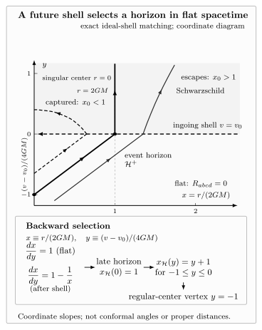
In the ideal null-shell model, matching at $v=v_0$, $r=2GM$ selects a horizon beginning at the regular center at $v_0-4GM$. Its earlier segment lies in flat spacetime. The neighboring rays are sampled from the piecewise radial null equations. This is an advanced-coordinate plot, not a Penrose diagram: displayed angles and separations are not conformal angles or proper distances.

This does not mean that the horizon exerts an influence backward in time. The metric and matter still satisfy local evolution equations. Teleology describes how a globally defined set is selected after the full solution is known, just as “the last zero of a function” depends on values at later arguments without causing earlier values.

Achronality and null generators

The escape region is a past set. Its boundary is therefore an achronal boundary and, under the usual horizon hypotheses, a future causal horizon. It is closed, locally Lipschitz, and ruled by future-directed null geodesics with no future endpoints on the horizon. Generators may have past endpoints where they join, and differentiability can fail there. These conclusions come from causal boundary theory, not from assuming a smooth null level set. The structural results are summarized in Minguzzi 2019, §2.14, pp. 59–64 and developed on Achronal Boundaries and Null Generators.

The words “no future endpoint on the horizon” do not assert future affine completeness. A generator might encounter an endpoint of the spacetime, and global theorems require additional predictability and regularity assumptions to control that possibility. Nor does null generation guarantee smoothness. At merger or formation points, several generators can enter through a crease set, as discussed on Horizon Regularity, Caustics, and Crease Sets.

Global and quasi-local boundaries are different

A trapped surface is diagnosed by the signs of two null expansions on a compact codimension-two surface. An apparent horizon is slicing dependent. Neither definition mentions $\mathscr I^+$, whereas the event horizon cannot be defined without it. In a collapse spacetime the event horizon can begin before any trapped surface occurs, as the thin-shell calculation already suggests. Conversely, implications from trapped surfaces to a black-hole region require energy, causality, completeness, and asymptotic hypotheses; they are not definitions.

An event horizon also need not be a Killing horizon. In a stationary solution the two may coincide under appropriate hypotheses and normalization, but a dynamical event horizon has no reason to be generated by a Killing field. The comparative taxonomy, equilibrium geometry, surface gravity, and mechanics belong to Event Horizons in the Horizon Taxonomy and the surrounding Black-Hole Geometry volume. Here the exact global causal definition is primary.

Finally, the asymptotically flat formula does not transfer unchanged to every setting. In de Sitter spacetime future conformal infinity is spacelike; in anti-de Sitter spacetime the conformal boundary is timelike and boundary conditions affect evolution. One must first specify the relevant accessible boundary and its causal problem, then define a relative black-hole region. A symbol $r=\text{constant}$ or a vanishing metric coefficient is never sufficient.

Exercises

For the thin-shell model above, derive the flat-region event-horizon generator and its starting advanced time. Then explain which information in the calculation is local and which is global.

Solution

After the shell settles to Schwarzschild, the late event horizon is $r=2GM$. Continuity at the shell fixes the relevant outgoing null ray to pass through $(v_0,2GM)$. In the flat interior, integrating $dr/dv=1/2$ yields

$$r(v)-2GM=\frac{v-v_0}{2}.$$

Setting $r=0$ gives $v=v_0-4GM$. The differential equation and the flatness of the pre-shell region are local facts. Selecting which outgoing ray is the event-horizon generator requires the future condition that it asymptote to the boundary of $J^-(\mathscr I^+)$. Without knowing the shell’s later mass and fate, the integration constant—and hence the earlier horizon location—cannot be chosen.

References

• Chruściel, Piotr T. “Black Holes.” Lecture Notes in Physics 604, 61–102 (2002). arXiv.
• Frauendiener, Jörg. “Conformal Infinity.” Living Reviews in Relativity 7, article 1 (2004). DOI.
• Gholizadeh Siahmazgi, Shohreh, Paul R. Anderson, Raymond D. Clark, and Alessandro Fabbri. “Stress-energy Tensor for a Quantized Scalar Field in a Four-Dimensional Black Hole Spacetime that Forms From the Collapse of a Null Shell.” Contribution to the Sixteenth Marcel Grossmann Meeting (2021). arXiv:2111.14764.
• Minguzzi, Ettore. “Lorentzian Causality Theory.” Living Reviews in Relativity 22, article 3 (2019). DOI.