Covariant Presymplectic Current

The covariant presymplectic current pairs two linearized perturbations without choosing a time coordinate or performing a 3+1 Legendre transform. It is the antisymmetrized second variation of the boundary term in the Lagrangian variation. On a solution, and for perturbations satisfying the linearized field equations, this local current is closed; its integral over a hypersurface is the presymplectic form, subject to convergence and boundary-flux conditions.

Required background. The Gibbons–Hawking–York Boundary Term supplies the variational role of gravitational boundary terms; Presymplectic Potentials and Currents supplies field-space variations and differential-form currents; and Killing Fields and Isometry Groups supplies infinitesimal diffeomorphisms.

Helpful background. The Einstein Equation supplies the equations of motion; Hypersurface Normals and Tangential Projectors supplies hypersurface orientation; and Formulations of General Relativity locates the construction within this volume.

Lagrangian variation and potential

Let $\phi$ denote all dynamical fields and let the Lagrangian be an $n$-form $L[\phi]$. After integration by parts, its first variation has the form

$$\delta L =E(\phi)\!\cdot\!\delta\phi+d\Theta(\phi;\delta\phi).$$

Here $E=0$ denotes the Euler–Lagrange equations and the $(n-1)$-form $\Theta$ is linear in the perturbation. It is called the presymplectic potential current, not a phase-space one-form at a single point: it is simultaneously a spacetime form and a field-space one-form.

For four-dimensional Einstein gravity,

$$L=\frac{1}{16\pi G}(R-2\Lambda)\epsilon,$$

and one covariant choice for $h_{ab}=\delta g_{ab}$ is

$$\Theta_{abc}(g;h) =\frac{1}{16\pi G}\epsilon_{dabc} \left(\nabla_eh^{de}-\nabla^dh\right), \qquad h=g^{ab}h_{ab}.$$

Here $h^{ab}=g^{ac}g^{bd}h_{cd}$ denotes the raised covariant perturbation, so $\delta g^{ab}=-h^{ab}$. Confusing these two tensors reverses the potential.

Iyer and Wald derive the general variational decomposition and this Einstein potential in Iyer and Wald 1994, §3, eqs. (20)–(23), and §5, eqs. (61)–(62), pp. 6–12, PDF.

Antisymmetrized second variation

Fix the sign convention used throughout this site:

$$\omega(\phi;\delta_1\phi,\delta_2\phi) =\delta_2\Theta(\phi;\delta_1\phi) -\delta_1\Theta(\phi;\delta_2\phi).$$

Thus $\omega$ is an $(n-1)$-form on spacetime and a two-form on field space. It is antisymmetric:

$$\omega(\delta_2,\delta_1)=-\omega(\delta_1,\delta_2).$$

Some references reverse the order of the two terms. Every later Hamiltonian and flux formula must be translated if that convention is used. The definition here matches Iyer and Wald 1994, §3, eqs. (44)–(45), pp. 9–10, PDF.

A finite-dimensional check fixes the Hamiltonian ordering without relying on a name for the convention. For a mechanical potential $\Theta=p\,\delta q$, this definition gives

$$\Omega(\delta_1,\delta_2) =\delta_1q\,\delta_2p-\delta_2q\,\delta_1p.$$

Hamilton’s equations $\dot q=\partial_pH$, $\dot p=-\partial_qH$ therefore satisfy $\Omega(X_H,\delta)=\delta H$, where $X_H=(\dot q,\dot p)$. The generator goes in the first slot. Equivalently $\Omega(\delta,X_H)=-\delta H$. The gravitational surface-charge identity below uses this same order.

For a hypersurface $\Sigma$ oriented by its future-directed unit normal, define

$$\Omega_\Sigma(\delta_1,\delta_2) =\int_\Sigma\omega(\delta_1,\delta_2).$$

It is called presymplectic because gauge directions can lie in its kernel. Only after imposing boundary conditions and quotienting the genuine degeneracies does one obtain a symplectic phase space. Lee and Wald develop this solution-space construction and its constraint-generated degeneracies in Lee and Wald 1990, §§2–4, pp. 727–735.

The diagram separates two questions about the integrated current. Follow the boundary-flux branch to decide whether it depends on the slice; follow the kernel branch to decide which transformations are redundancies. Passing one test does not imply passing the other.

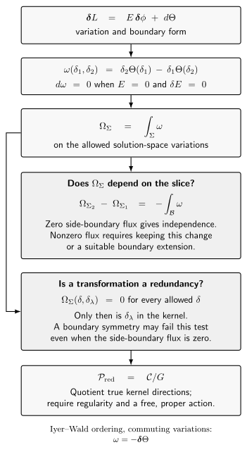
After forming the presymplectic integral, ask two separate questions. Boundary flux controls its change between slices; pairing with every allowed variation determines whether a transformation lies in its kernel. A boundary symmetry can have nonzero pairing even when flux vanishes. Quotient only true kernel directions under the stated regularity hypotheses. Schematic process diagram.

Why the current is closed

Apply two commuting variations to $L$ and subtract them. The bulk and boundary pieces give

$$d\omega =\delta_1E\!\cdot\!\delta_2\phi -\delta_2E\!\cdot\!\delta_1\phi.$$

If the background satisfies $E=0$ and both perturbations are tangent to the solution space, so that $\delta_1E=\delta_2E=0$, then

$$d\omega=0.$$

For two hypersurfaces $\Sigma_1$ and $\Sigma_2$ bounding a spacetime region together with a lateral boundary $\mathcal B$, Stokes’ theorem yields

$$\Omega_{\Sigma_2}-\Omega_{\Sigma_1} =-\int_{\mathcal B}\omega,$$

with the displayed sign fixed by the induced boundary orientation. Hypersurface independence therefore requires vanishing total symplectic flux through the lateral boundary, or a boundary contribution that consistently accounts for that flux. Local closedness alone is not enough.

Exact-form ambiguities

Adding an exact form to the Lagrangian, $L\mapsto L+d\mu$, changes $\Theta\mapsto\Theta+\delta\mu$. This term cancels from the antisymmetrized second variation when variations commute. A second ambiguity,

$$\Theta\mapsto\Theta+dY(\phi;\delta\phi),$$

changes $\omega$ by an exact spacetime form. Its integral changes by a corner term on $\partial\Sigma$. Consequently a harmless bulk ambiguity can be physically relevant when boundaries or asymptotic ends are present. A charge calculation must state the action, potential prescription, boundary conditions, and corner terms together.

Common pitfalls

Closed does not mean exact globally. Cohomology and boundary conditions can prevent a global potential even when $d\omega=0$.

On shell is required twice. The background must solve the equations, and the two variations must solve the linearized equations for current conservation.

Presymplectic is not yet reduced phase space. Diffeomorphisms that vanish appropriately at the boundary are candidate degeneracies; boundary-active diffeomorphisms need separate treatment.

Exercise: conservation between slices

Let $\delta_1g$ and $\delta_2g$ satisfy the linearized Einstein equation in a region bounded by $\Sigma_1$, $\Sigma_2$, and $\mathcal B$. Show the condition under which the two hypersurface integrals agree.

Solution

The linearized equations imply $d\omega=0$. Stokes’ theorem gives

$$0=\int_{\partial V}\omega =\Omega_{\Sigma_2}-\Omega_{\Sigma_1} +\int_{\mathcal B}\omega.$$

Therefore the two bare bulk integrals agree precisely when the integrated symplectic flux through $\mathcal B$ vanishes. Pointwise vanishing is sufficient but not necessary: different boundary components can cancel in the total. If a boundary or corner contribution is added to the presymplectic form, its change must instead be included explicitly; conservation of that extended form does not imply equality of the bare bulk integrals.

References

• Iyer, Vivek, and Robert M. Wald. “Some Properties of Noether Charge and a Proposal for Dynamical Black Hole Entropy.” Physical Review D 50, no. 2 (1994): 846–864. DOI; Open PDF.
• Lee, Joohan, and Robert M. Wald. “Local Symmetries and Constraints.” Journal of Mathematical Physics 31, no. 3 (1990): 725–743. DOI.