Model Error and Scientific Bias

A waveform residual is scientifically consequential according to its direction in model space, not only its norm. Error parallel to parameter tangents can be absorbed by shifting inferred parameters; equal-norm orthogonal error can leave the leading parameter estimate unchanged while degrading fit or exposing model inadequacy. Signal strength, PSD, priors, parameterization, calibration, and model flexibility change that geometry. As of the 2026-08-18 evidence cutoff, no universal mismatch threshold determines bias across all sources and scientific tasks.

Required background. Probability and Statistical Inference supplies likelihood expansion, Fisher geometry, priors, coverage, and bias diagnostics.

Helpful background. Einstein Equations supplies the physical waveform family. Waves, Green Functions, and Geometric Optics supplies weighted signal geometry. Gravitational Radiation and Waveforms supplies model residuals and match. Computational Relativity supplies reference and numerical uncertainties.

Linearized likelihood geometry

Let the true noiseless signal be

$$h_*=h_m(\theta_0)+\delta h,$$

where $\delta h$ is truth minus model at physical parameters $\theta_0$. With a declared Gaussian-noise inner product, expand

$$h_m(\theta_0+\Delta\theta) \simeq h_m(\theta_0) +\partial_i h\,\Delta\theta^i.$$

The residual is $r=\delta h-\partial_i h\,\Delta\theta^i$. Differentiating $\lVert r\rVert^2$ with respect to each fitted parameter sets $(\partial_jh\mid r)=0$. Hence the normal equations are $\Gamma_{ji}\Delta\theta^i=(\partial_jh\mid\delta h)$, giving the first-order theoretical displacement

$$\Delta\theta^i_{\mathrm{sys}} =(\Gamma^{-1})^{ij} (\partial_jh\mid\delta h), \qquad \Gamma_{ij}=(\partial_i h\mid\partial_j h).$$

This tangent-space result and its domain are derived in Cutler and Vallisneri 2007, §II.A–B, pp. 2–4, PDF. Here $\theta^i$ must include every direction optimized in the stated fit. If amplitude or normalization, arrival time, and phase are maximized, their tangents must appear in the full Gram/Fisher matrix or be projected out separately before the displayed intrinsic block is used. For a real detector channel, the first two are proportional to $h$ and $\partial_t h$. A constant phase applied to the positive-frequency representation has tangent $\operatorname{Re}(i h_+)$, where $h_+$ is the analytic signal defined in Match, Mismatch, and Alignment; it is not multiplication of the real strain by $i$. The result also assumes a locally linear waveform manifold, invertible projected geometry, fixed weighting, sufficiently informative likelihood, and no dominating prior boundary.

Parallel and orthogonal error

The figure shows the least-squares construction in a two-dimensional slice of waveform space. Start at the model with the physical parameters, then move along a fitted parameter direction as far as the data allow. The shortest remaining displacement is perpendicular to that direction in the chosen noise-weighted geometry.

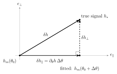
Truth-minus-model error separates into a fitted waveform displacement $\delta h_\parallel$ and a remaining residual $\delta h_\perp$. The axes are locally whitened waveform directions, not spatial coordinates. This schematic assumes a locally linear model, a fixed positive noise weighting, and all declared fitted directions; it does not represent a nonlinear posterior.

Project

$$\delta h_\parallel =\partial_i h(\Gamma^{-1})^{ij} (\partial_jh\mid\delta h), \qquad \delta h_\perp=\delta h-\delta h_\parallel.$$

The parallel component produces the leading shifts in the full fitted parameter set. The orthogonal component satisfies $(\partial_i h\mid\delta h_\perp)=0$ for every included intrinsic and nuisance direction and cannot be absorbed at first order. It instead contributes to the best-fit residual and model checking. Omitting an optimized direction would misclassify a removable component—for example, a pure amplitude rescaling—as residual error. Nonlinear curvature of the manifold mixes these roles at larger errors.

For signal norm $\rho=\lVert h\rVert$ and a small error after normalization and every declared time, phase, and parameter alignment, mismatch is approximately

$$\mathfrak m\simeq \frac{\lVert\delta h_\perp\rVert^2}{2\rho^2}.$$

The same mismatch therefore corresponds to a larger absolute residual at larger $\rho$. A fixed mismatch cannot be a signal-strength-independent distinguishability rule.

Norm standards are sufficient, not universal

The absolute condition $\lVert\delta h\rVert\lt1$ provides conservative sufficient control in the declared Gaussian, fixed-PSD, locally linear problem. Practical amplitude/phase conditions can be stronger. The measurement standard and its assumptions are given in Lindblom, Owen, and Brown 2008, §II.A, eqs. (4)–(9), p. 3, PDF.

Within the Fisher approximation this statement has a precise meaning. Because the fitted waveform shift is the orthogonal projection $\delta h_\parallel$,

$$\Delta\theta^i_{\rm sys}\Gamma_{ij}\Delta\theta^j_{\rm sys} =\lVert\delta h_\parallel\rVert^2 \le\lVert\delta h\rVert^2.$$

For any locally linear parameter combination $q=q_i\theta^i$, its statistical variance is $\sigma_q^2=q_i(\Gamma^{-1})^{ij}q_j$. Cauchy–Schwarz in parameter space then gives

$$\frac{\lvert\Delta q_{\rm sys}\rvert}{\sigma_q} \le\lVert\delta h_\parallel\rVert \le\lVert\delta h\rVert.$$

An absolute error norm below one therefore cannot conceal a many-standard-deviation linearized bias simply by pointing along a sensitive parameter. A small fractional error $\lVert\delta h\rVert/\rho$ or a small optimized mismatch is different: neither bounds that absolute norm without the signal strength and the removed directions.

The sufficient bound is not necessary for every task. A large error orthogonal to a particular parameter tangent may produce no leading shift of that parameter, while leaving an obvious residual. Conversely, absorbing a tangent error improves the fit by moving the inferred parameters; it is not protection against bias. Priors, nonlinearities, boundaries, or a different scientific observable require their own analysis.

Results and interpretations through 2026-08-18

The literature and method status through 2026-08-18 supports conditional diagnostics, not one universal mismatch rule. A current review separates waveform mismodeling from instrumental and astrophysical systematics and emphasizes that their relevance changes with source, band, and signal strength Yunes, Siemens, and Yagi 2025, §3.3.3, pp. 49–50, PDF.

evidence or method	supported result or use	scope, limitation, or missing control
Norm-based sufficient standards	Bound total weighted discrepancy under declared PSD, band, response, and signal scale Lindblom, Owen, and Brown 2008, §II.A, PDF	Gives a worst-case linearized bias bound; does not determine the actual error direction or apply unchanged outside its assumptions
Tangent-space Fisher estimate	Predicts first-order parameter displacement from projections $(\partial_i h\mid\delta h)$ Cutler and Vallisneri 2007, §II.A–B, pp. 2–4, PDF	Requires local linearity, invertible geometry, high-information likelihood, and weak prior boundaries
Injection and operational-coverage studies	Test end-to-end recovery and whether approximate credible sets attain declared coverage Pürrer and Haster 2020, §§II–IV, PDF; Mao et al. 2024, §§III–V, PDF	Conclusions depend on injection distribution, noise, priors, model pair, and coverage estimator; a proof-of-principle calibration is not universal coverage
NR-calibration-uncertainty marginalization	Samples a fitted distribution for waveform calibration parameters rather than fixing one best fit Pompili, Buonanno, and Pürrer 2025, §§III–IV, PDF	The uncertainty model, training residuals, and correlations must themselves be validated; the cited tests use selected aligned-spin loud injections
Surrogate cross-validation	Measures held-out reconstruction error and maps failure inside a declared calibration domain Field et al. 2014, §IV, PDF; Varma et al. 2019, §VII, PDF	Common reference error is not exposed; selected norm, split, domain density, and extrapolation control the result
Population bias scan	Shows which parameters and sources expose or absorb error for one population and model pair Kapil et al. 2024, §§II–V, PDF	A linear-signal population study does not determine event-level nonlinear posteriors or transfer to another population, detector, or model pair

For the simulated events with network SNR $\ge100$, the population scan estimated a bias larger than one statistical standard deviation in $3.7\%$–$18.3\%$ of cases, depending on the parameter. This comparison used IMRPhenomD and IMRPhenomXAS with a specified two-Cosmic-Explorer plus Einstein-Telescope network Kapil et al. 2024, §IV, Figure 2, p. 5, PDF. Most events in that selected subset remained below the study’s one-sigma threshold for each parameter. That is a conditional linear-signal estimate, not proof that those events have no waveform bias; neither fraction transfers automatically to another population, detector configuration, or model pair.

The competing positions are a conditional use of mismatch and projected-error criteria versus the stronger, unsupported claim that one threshold decides bias across detectors, priors, source populations, waveform models, and scientific questions. The latter is not settled by existing norm derivations. Reliable claims require a specified data class, parameter regime, waveform model, PSD, prior, and target quantity.

Equal-norm counterexample

Let $e_\parallel=\partial_\theta h/\sqrt{\Gamma}$ be a unit tangent and $e_\perp$ a unit orthogonal direction. Compare

$$\delta h_1=\epsilon e_\parallel, \qquad \delta h_2=\epsilon e_\perp.$$

Both have norm $\epsilon$. For the first,

$$\Delta\theta_{1}=\frac{\epsilon}{\sqrt\Gamma}, \qquad \delta h_{1,\perp}=0.$$

For the second,

$$\Delta\theta_{2}=0, \qquad \lVert\delta h_{2,\perp}\rVert=\epsilon.$$

Thus equal norms yield different leading parameter shifts and best-fit residuals. With several correlated parameters, the Fisher eigenvectors and prior directions replace this two-dimensional picture.

SNR, PSD, prior, and parameterization

For a fixed fractional waveform error, scaling source amplitude by $A$ makes both $\Gamma$ and $(\partial h\mid\delta h)$ scale as $A^2$, so the leading absolute parameter displacement can remain roughly constant while statistical widths shrink as $1/A$. Its significance therefore grows with SNR even when mismatch is unchanged.

Changing the PSD rotates and stretches waveform space, altering tangent projections. A narrow prior can suppress a Fisher-predicted shift and move tension into residual structure or a boundary; a broad prior permits more absorption. Reparameterization changes numerical coordinate bias through the Jacobian even though a correctly transformed physical prediction is invariant. Event-specific judgments require the actual likelihood, priors, calibration, and model family.

Beyond the Fisher approximation

Injection studies can sample nonlinear degeneracies, multimodal likelihoods, boundaries, and noise realizations. Pürrer and Haster’s zero-noise recoveries demonstrate how detector configuration and waveform pair change bias, while Mao and collaborators calibrate operational coverage for approximate posteriors in a controlled proof of principle Pürrer and Haster 2020, §§II–IV, PDF; Mao et al. 2024, §§III–V, PDF. Coverage tests ask whether repeated credible sets contain injected parameters at their stated frequency under a declared data-generating process. Posterior predictive residuals ask whether the fitted model leaves structured data. Neither is model independent: injection populations, reference waveforms, priors, noise, and calibration must be varied.

Waveform calibration uncertainty can be marginalized when a defensible conditional error model exists; one concrete construction samples distributions for EOB NR-calibration parameters during inference Pompili, Buonanno, and Pürrer 2025, §§III–IV, PDF. Surrogate validation instead holds out waveforms and measures reconstruction error in a declared norm Field et al. 2014, §IV, PDF; Varma et al. 2019, §VII, PDF. Inflating uncertainty without validating its correlation structure can conceal systematic trends. Reference-model disagreement is evidence about the chosen ensemble of models, not a probability law over unknown truth.

Boundaries and unresolved status

This research bridge provides criteria and counterexamples, not current detector requirements or event-specific parameter biases. Those empirical applications are treated in Gravitational-Wave Astronomy. The norm bound is mathematically useful within its stated assumptions; extending a single mismatch threshold to nonlinear, prior-sensitive problems across all source classes is not established by the evidence reviewed here.

What could change the conclusion

The interpretation could change after new validated coverage studies expose a failure or domain of a stated criterion, after revised mission requirements change a declared accuracy task, after public waveform comparisons supply independently controlled residual directions, or after a counterexample invalidates the tangent-space or norm interpretation used here. The review must retain explicit PSD, SNR, prior, parameterization, and calibration assumptions.

Exercises

1. Same mismatch, different signal strength. If $\mathfrak m=10^{-4}$, estimate $\lVert\delta h_\perp\rVert$ for $\rho=20$ and $\rho=100$.

Solution

Using $\lVert\delta h_\perp\rVert\simeq\rho\sqrt{2\mathfrak m}$ gives

$$\sqrt{2\mathfrak m}=\sqrt{2\times10^{-4}} \simeq0.01414.$$

Therefore the residual norms are about $0.283$ and $1.414$, respectively. The mismatch is identical, but the higher-SNR signal has a residual of order unity in the weighted geometry. This is why a fixed mismatch cannot encode universal distinguishability.

2. Rotate the error direction. Let $\delta h(\alpha)=\epsilon(\cos\alpha\,e_\parallel+\sin\alpha\,e_\perp)$. Find the leading shift and residual norm.

Solution

Projection gives

$$\Delta\theta=\frac{\epsilon\cos\alpha}{\sqrt\Gamma}, \qquad \lVert\delta h_\perp\rVert =\epsilon\lvert\sin\alpha\rvert.$$

The total norm remains $\epsilon$ for every $\alpha$, yet the bias-residual balance varies continuously. At $\alpha=0$ the error is fully absorbed at first order; at $\alpha=\pi/2$ it produces no first-order shift and remains entirely in the residual.

References

• Cutler, Curt, and Michele Vallisneri. “LISA Detections of Massive Black Hole Inspirals: Parameter Extraction Errors Due to Inaccurate Template Waveforms.” Physical Review D 76 (2007): 104018. DOI. Open PDF.
• Field, Scott E., Chad R. Galley, Jan S. Hesthaven, Jason Kaye, and Manuel Tiglio. “Fast Prediction and Evaluation of Gravitational Waveforms Using Surrogate Models.” Physical Review X 4 (2014): 031006. DOI. Open PDF.
• Kapil, Veome, Luca Reali, Roberto Cotesta, and Emanuele Berti. “Systematic Bias from Waveform Modeling for Binary Black Hole Populations in Next-Generation Gravitational Wave Detectors.” Physical Review D 109 (2024): 104043. DOI. Open PDF.
• Lindblom, Lee, Benjamin J. Owen, and Duncan A. Brown. “Model Waveform Accuracy Standards for Gravitational Wave Data Analysis.” Physical Review D 78 (2008): 124020. DOI. Open PDF.
• Mao, Ruiting, Jeong Eun Lee, Ollie Burke, Alvin J. K. Chua, Matthew C. Edwards, and Renate Meyer. “Calibrating Approximate Bayesian Credible Intervals of Gravitational-Wave Parameters.” Physical Review D 109 (2024): 083002. DOI. Open PDF.
• Pompili, Lorenzo, Alessandra Buonanno, and Michael Pürrer. “Accounting for Numerical-Relativity Calibration Uncertainty in Gravitational-Wave Modeling and Inference.” Physical Review D 112 (2025): 044062. DOI. Open PDF.
• Pürrer, Michael, and Carl-Johan Haster. “Ready for What Lies Ahead? Gravitational Waveform Accuracy Requirements for Future Ground-Based Detectors.” Physical Review Research 2 (2020): 023151. DOI. Open PDF.
• Varma, Vijay, Scott E. Field, Mark A. Scheel, Jonathan Blackman, Lawrence E. Kidder, and Harald P. Pfeiffer. “Surrogate Model of Hybridized Numerical Relativity Binary Black Hole Waveforms.” Physical Review D 99 (2019): 064045. DOI. Open PDF.
• Yunes, Nicolás, Xavier Siemens, and Kent Yagi. “Gravitational-Wave Tests of General Relativity with Ground-Based Detectors and Pulsar-Timing Arrays.” Living Reviews in Relativity 28 (2025): 3. DOI. Open PDF.