Tidal Response to a Passing Wave

A passing gravitational wave is measured through relative acceleration, not through the coordinate motion of one test mass. In a local freely falling frame, the electric part of the Riemann tensor drives neighboring geodesics. For wavelengths long compared with the apparatus, integrating that tidal acceleration reproduces the familiar plus and cross deformations of a ring of particles and the differential length change of orthogonal arms.

Required background. Weak-Field Gravity is used to compute the linearized curvature from a metric perturbation. Waves, Green Functions, and Geometric Optics supplies the plane-wave and long-wavelength approximations.

Helpful background. Einstein Equations identifies the vacuum regime in which the wave propagates. Equivalence Principles and Gravitational Measurement supplies local inertial frames, freely falling observers, and tidal measurements.

Curvature in the observer’s local frame

Let a central freely falling observer have four-velocity $U^\mu$, and let $\xi^\mu$ connect that worldline to a neighboring geodesic. With the site’s curvature convention, geodesic deviation is

$$\frac{D^2\xi^\mu}{d\tau^2} =-R^\mu{}_{\alpha\nu\beta} U^\alpha\xi^\nu U^\beta.$$

Choose an orthonormal tetrad transported along the central geodesic. At the reference event, $U^{\hat\mu}=(1,0,0,0)$ and the spatial equation becomes

$$\frac{d^2\xi^{\hat i}}{d\tau^2} =-R^{\hat i}{}_{\hat0\hat j\hat0}\,\xi^{\hat j}.$$

The symmetric matrix

$$\mathcal E_{\hat i\hat j}=R_{\hat0\hat i\hat0\hat j}$$

is the electric tidal tensor. In a vacuum region it is trace free because $R_{\hat0\hat0}=0$. Its components in the transported tetrad are directly operational: they give relative acceleration per unit separation.

For a linearized TT perturbation on Minkowski spacetime,

$$R^{(1)}_{0i0j}=-\frac12\ddot h^{\mathrm{TT}}_{ij},$$

so, to first order in the wave amplitude,

$$\ddot\xi^i=\frac12\ddot h^{\mathrm{TT}}_{ij}\xi_0^j.$$

For particles initially at relative rest, $\xi_0^j$ is the constant zeroth-order separation. It can be used on the right-hand side because replacing it by the perturbed separation would change the result only at second order. Flanagan and Hughes derive this local-observer response and distinguish it from coordinate displacement in Flanagan and Hughes 2005, §3, eqs. (3.6)–(3.12), pp. 14–16, PDF.

Integrating the long-wavelength response

Assume that the apparatus size $L$ is much smaller than the reduced wavelength $\lambda_{\rm red}=\omega^{-1}$ of the relevant Fourier components. Before the pulse, take $h_{ij}^{\mathrm{TT}}=\dot h_{ij}^{\mathrm{TT}}=0$ and $\dot\xi^i=0$. Integrating twice gives, to first order in amplitude and leading order in $L/\lambda_{\rm red}$,

$$\xi^i(t) =\left(\delta^i{}_j+\frac12h^{\mathrm{TT}\,i}{}_j(t)\right)\xi_0^j.$$

The neglected displacement scales as $O(h^2L)$ from nonlinear amplitude corrections and, conservatively, $O(hL^2/\lambda_{\rm red})$ from spatial variation across a finite apparatus. These are length errors, and both vanish when the incident wave vanishes. Different initial strain or relative velocity adds the corresponding integration constants; curvature alone does not set them.

For propagation along $+z$,

$$h^{\mathrm{TT}}_{ij} =\begin{pmatrix} h_+&h_\times&0\\ h_\times&-h_+&0\\ 0&0&0 \end{pmatrix}.$$

A particle initially at $(x_0,y_0)$ in the transverse plane therefore moves, in the local proper frame, by

$$\delta x=\frac12(h_+x_0+h_\times y_0), \qquad \delta y=\frac12(h_\times x_0-h_+y_0).$$

For a pure plus wave, the $x$ and $y$ axes are alternately stretched and compressed. For a pure cross wave, the principal axes are rotated by $45^\circ$. The transverse area changes only at second order because the first-order deformation is trace free.

The figure compares two opposite phases of each polarization. Follow the initially circular dashed ring: the plus wave stretches along the coordinate axes, while the cross wave stretches along the diagonals.

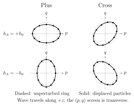
Long-wavelength tidal response of particles initially at relative rest, using $\boldsymbol x=(I+h^{\rm TT}/2)\boldsymbol x_0$. Each polarization is shown at $h_A=\pm h_0$ with the other polarization zero; the dashed circle is the initial ring. The amplitude $h_0=0.4$ is exaggerated for visibility and the drawing is schematic. The linear map preserves area only to first order; its finite-amplitude area change is not a prediction of a second-order calculation.

The same physics can look different in TT coordinates. Freely falling particles initially at rest keep fixed spatial coordinate labels to first order, while the spatial metric changes their proper separations. In a Fermi-like local frame the spatial metric is locally Euclidean at the central worldline and the particles’ coordinates move. Both descriptions give the same curvature and measured distance; treating either coordinate picture as uniquely physical creates a false gauge paradox.

Arm-length response

Let an arm have unperturbed length $L$ and unit direction $a^i$ in the transverse screen. In the long-wavelength, freely suspended limit,

$$\frac{\delta L_a}{L} =\frac12a^i a^j h^{\mathrm{TT}}_{ij}.$$

For orthogonal $x$ and $y$ arms,

$$\frac{\delta L_x}{L}=\frac12h_+, \qquad \frac{\delta L_y}{L}=-\frac12h_+,$$

and their differential strain is

$$\frac{\delta L_x-\delta L_y}{L}=h_+.$$

This is a local, low-frequency geometric result. When $L/\lambda_{\rm red}$ is not negligible, the field changes while light propagates along the arm, and the observable must be computed from photon emission, propagation, and reception. Suspension dynamics, optical cavities, calibration, and noise also lie beyond this page. They belong to the detector treatment in Gravitational-Wave Astronomy.

Likewise, the response does not determine the nonlinear compact-binary dynamics that produced $h_{ij}^{\mathrm{TT}}$. That source problem belongs to Relativistic Two-Body Dynamics; here the waveform is accepted as specified incident radiative data.

Gauge-invariance check

Under the chapter’s passive convention, $h_{\mu\nu}\mapsto h_{\mu\nu}-2\partial_{(\mu}\xi_{\nu)}$, the linearized Riemann tensor is unchanged. The tidal prediction is therefore unchanged even though the coordinate positions and individual metric components may differ. This gives a practical diagnostic:

1. construct $R^{(1)}_{0i0j}$ from the proposed perturbation;
2. add a pure-gauge perturbation and recompute it;
3. verify exact cancellation of every $\xi^\mu$ contribution before interpreting a particle pattern.

A particle plot derived directly from coordinate motion without this check can display gauge motion rather than a gravitational wave.

Common pitfalls

Saying gravity is transformed away along a worldline. Connection coefficients can vanish on the central geodesic, but curvature and relative acceleration remain. The equivalence principle is precisely compatible with tidal measurement.

Using the ring picture outside the long-wavelength limit. A single tidal matrix describes the whole apparatus only when spatial variation across it is negligible. Finite-arm response requires light propagation through the varying field.

Equating zero late-time curvature with zero observable history. Curvature is proportional to two derivatives of strain. A burst may leave a persistent displacement memory after its local curvature has returned to zero.

Exercises

1. Area of a particle ring. A pure plus wave maps an initially circular ring of radius $R$ to semiaxes $R(1+h_+/2)$ and $R(1-h_+/2)$. Show that its area is unchanged at first order.

Solution

The deformed area is

$$A=\pi R^2\left(1+\frac{h_+}{2}\right) \left(1-\frac{h_+}{2}\right) =\pi R^2\left(1-\frac{h_+^2}{4}\right).$$

There is no term linear in $h_+$. This is the geometric consequence of the trace-free screen deformation: one principal direction expands by the amount the orthogonal direction contracts. The $O(h_+^2)$ change lies beyond linearized response.

2. A rotated arm. Let $a^i=(\cos\alpha,\sin\alpha,0)$. Compute its fractional length response to both polarizations.

Solution

Contracting the arm direction twice with the TT matrix gives

$$\frac{\delta L_a}{L} =\frac12\left(h_+\cos2\alpha+h_\times\sin2\alpha\right).$$

The double angle is the spin-2 signature. A $45^\circ$ rotation exchanges sensitivity to plus and cross, while a $90^\circ$ rotation reverses the sign of the response. No new polarization is produced by rotating the arm.

References

• Flanagan, Éanna É., and Scott A. Hughes. “The Basics of Gravitational Wave Theory.” New Journal of Physics 7 (2005): 204. DOI. Open PDF.