Michelson Interferometer Response

An ideal Michelson interferometer turns a passing gravitational wave into a differential optical phase: the two arms sample different projections of the spatial strain, and the beams compare those projections when they recombine. In the small-antenna limit the entire geometric response is the contraction $D^{ij}h_{ij}$ with a trace-free detector tensor. This page derives that result for freely suspended, equal arms and identifies what must be added before it describes a real calibrated channel.

Required background. The Wave Equation and Characteristics supplies plane-wave phase, characteristics, and the approximation that the field varies negligibly across one light path.

Helpful background. Gravitational Radiation and Waveforms fixes the strain and polarization conventions used here. Probability and Inference for Gravity becomes useful when response and calibration uncertainties are introduced.

Light paths in a weak tensor wave

Work to first order about Minkowski spacetime,

$$ds^2=-c^2dt^2+\left(\delta_{ij}+h_{ij}^{\mathrm{TT}}\right)dx^i dx^j,$$

and let $\boldsymbol u$ be a unit vector along one arm of unperturbed length $L$. In TT coordinates the freely falling beam splitter and end mirror remain at fixed coordinate positions, while their instantaneous proper separation changes. If the gravitational wavelength is much longer than the arm,

$$\frac{\delta L_{\boldsymbol u}(t)}{L} =\frac12 u^iu^j h_{ij}^{\mathrm{TT}}(t).$$

This is the twice-integrated tidal response, with the initial relative displacement and velocity fixed by the unperturbed freely falling configuration. In the time coordinate $t$ used above, the curvature statement is $R_{titj}^{(1)}=-\ddot h_{ij}^{\mathrm{TT}}/2$; with $x^0=ct$ it is $R_{0i0j}^{(1)}=-\ddot h_{ij}^{\mathrm{TT}}/(2c^2)$. Both give the relative acceleration $\ddot\xi^i=\tfrac12\ddot h^i{}_j\xi^j$ at leading order. The bridge from curvature to strain is derived in Flanagan and Hughes 2005, §3, Eqs. (3.5)–(3.13), PDF.

A monochromatic laser of angular frequency $\omega_0$ accumulates the round-trip phase $2\omega_0L/c$. Therefore a slowly varying arm displacement produces

$$\delta\phi_{\boldsymbol u}(t) =\frac{2\omega_0}{c}\,\delta L_{\boldsymbol u}(t).$$

The slowly varying qualification matters twice: the wave must be nearly constant during the photon round trip, and the optical field must follow the changing arm without a cavity or readout bandwidth becoming important. Those two restrictions are relaxed separately on the finite-arm response and optical-cavity pages.

Differential response and detector tensor

Let the second arm point along the unit vector $\boldsymbol v$. The antisymmetric output compares the two round-trip phases,

$$\Delta\phi =\delta\phi_{\boldsymbol u}-\delta\phi_{\boldsymbol v} =\frac{2\omega_0L}{c}\,s(t),$$

where the dimensionless ideal strain channel is

$$s(t)=D^{ij}h_{ij}^{\mathrm{TT}}(t), \qquad D^{ij}=\frac12\left(u^iu^j-v^iv^j\right).$$

The factor $1/2$ is fixed by the single-arm relation. For equal arms, $D^i{}_i=0$: a common isotropic length change cancels at the differential port. For a right-angle interferometer, $\boldsymbol u\mathbin{\cdot}\boldsymbol v=0$ and

$$D^{ij}D_{ij}=\frac12.$$

More generally, if the opening angle is $\zeta$,

$$D^{ij}D_{ij}=\frac12\sin^2\zeta.$$

Thus the geometry itself supplies a response scale. It does not supply optical power, shot noise, control-loop gain, or a calibration model.

Resolving the wave on a polarization screen gives

$$h_{ij}^{\mathrm{TT}} =h_+e^+_{ij}+h_\times e^\times_{ij},$$

so the channel becomes

$$s=F_+h_++F_\times h_\times, \qquad F_A=D^{ij}e^A_{ij}.$$

The labels plus and cross depend on the chosen screen, but $s$ does not: a screen rotation transforms the component columns $(h_+,h_\times)$ and $(F_+,F_\times)$ by the same orthogonal spin-2 rotation, preserving their scalar product. This contraction is the starting point for the full antenna patterns derived on the polarization-response page.

A normalization check

The figure isolates the simplest geometry. Follow the returning light from each mirror to the beam splitter: the readout compares the two round trips, so opposite arm changes reinforce one another in the difference.

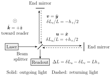
The differential response adds the opposite arm changes of a normally incident plus-polarized wave. The arm basis is aligned with the polarization axes. Equal-arm, freely falling, long-wavelength schematic, without optical cavities or control loops; ray offsets are for legibility and the drawing is not to scale.

Choose orthogonal arms $\boldsymbol u=\boldsymbol e_x$ and $\boldsymbol v=\boldsymbol e_y$, and let a wave propagate along $+z$. With

$$e^+_{ij}= \begin{pmatrix} 1&0&0\\ 0&-1&0\\ 0&0&0 \end{pmatrix}, \qquad e^\times_{ij}= \begin{pmatrix} 0&1&0\\ 1&0&0\\ 0&0&0 \end{pmatrix},$$

one obtains $F_+=1$ and $F_\times=0$. Hence $s=h_+$ and

$$\Delta\phi=\frac{2\omega_0L}{c}h_+.$$

For scale, $L=4\,\mathrm{km}$ and $h_+=10^{-21}$ give a differential displacement $\delta L_x-\delta L_y=Lh_+=4\times10^{-18}\,\mathrm m$. A laser wavelength $\lambda_0=1064\,\mathrm{nm}$ then gives $\Delta\phi=4\pi Lh_+/\lambda_0\simeq4.7\times10^{-11}$ radians for a bare Michelson. These are illustrative values, not a sensitivity claim; optical storage increases the phase response, while noise determines whether it can be measured.

Rotating the polarization screen by $45^\circ$ exchanges which named component is visible, but leaves the physical phase unchanged. Reversing either arm direction also leaves $D^{ij}$ unchanged because each arm enters quadratically.

The exact light-travel-time calculation reduces to this detector tensor when $fL/c\to0$; Romano and Cornish 2017, §5.2.3, Eqs. (5.29)–(5.32), PDF provides an independent derivation. Advanced ground-based detectors implement this geometry with arm cavities, recycling optics, control systems, and a calibrated readout rather than a bare Michelson; their optical architecture is documented in LIGO Scientific Collaboration 2015, §2 and Table 1, PDF.

What reaches an analysis

The ideal response $s=D:h$ is neither a photodiode count nor a released strain sample. A real chain has at least four maps:

$$h_{ij} \longrightarrow \Delta L_{\mathrm{free}} \longrightarrow d_{\mathrm{err}},d_{\mathrm{ctrl}} \longrightarrow d_{\rm calibrated} \longrightarrow \text{selected analysis data}.$$

Optical cavities and finite light travel modify the response; feedback distributes the free differential motion between residual and controlled motion; calibration reconstructs the strain channel, including its noise. Ideally $d_{\rm calibrated}=s+n$, where $s$ is the predicted detector strain and $n$ is equivalent strain noise. The released calibrated stream already contains that noise. Data-quality selection determines which samples enter a likelihood. Conflating adjacent stages hides a transfer function or an uncertainty.

For observational use, the detector, time interval, response version, calibration envelope, frequency band, and quality mask must all be fixed. The official public interface used by this volume is the GWOSC O4 technical record, as available on 2026-08-18. No O4 sensitivity or event claim is inferred on this page: its result is the stable geometric limit against which a versioned response product can be checked.

Common pitfalls

Treating $h_+$ as the detector output. A detector measures $F_+h_++F_\times h_\times$, followed by frequency-dependent instrument response and calibration. Only a special source direction and screen give $F_+=1$, $F_\times=0$.

Calling TT coordinates the observable. The operational quantity is differential light travel or phase. TT gauge makes the weak, freely falling calculation economical; curvature and the final phase comparison provide the invariant physical content.

Using the result when $fL/c$ is not small. Different photon-path segments then sample different wave phases. The constant tensor $D^{ij}$ must be replaced by a complex, direction- and frequency-dependent response.

Exercises

1. Opening-angle response. Show that an equal-arm Michelson with opening angle $\zeta$ satisfies $D^{ij}D_{ij}=\tfrac12\sin^2\zeta$. What happens as the arms become parallel?

Solution

Using $u^iu_i=v^iv_i=1$ and $u^iv_i=\cos\zeta$,

$$\begin{aligned} D^{ij}D_{ij} &=\frac14\left[(u^iu^j)(u_i u_j)+(v^iv^j)(v_i v_j) -2(u^iu^j)(v_i v_j)\right]\\ &=\frac14\left(1+1-2\cos^2\zeta\right) =\frac12\sin^2\zeta. \end{aligned}$$

For parallel arms, $\zeta=0$ and $D^{ij}=0$: both paths acquire the same first-order phase, so their difference contains no gravitational-wave signal.

2. From strain to optical phase. A right-angle bare Michelson faces a plus-polarized wave normally, with $h_+(t)=h_0\cos\Omega t$. Derive the differential phase in the small-antenna limit and identify two reasons this formula is not yet a calibrated detector model.

Solution

The normalization check gives $s=h_+$, hence

$$\Delta\phi(t)=\frac{2\omega_0L}{c}h_0\cos\Omega t.$$

The formula omits the optical-cavity and recycling response, and it assumes the wave phase is effectively constant during the round trip. It also omits feedback, sensing electronics, calibration uncertainty, and noise; naming any two of these missing layers answers the second part.

References

• Flanagan, Éanna É., and Scott A. Hughes. “The Basics of Gravitational Wave Theory.” New Journal of Physics 7 (2005): 204. DOI. Open PDF.
• Gravitational Wave Open Science Center. “O4 Technical Details.” Version available 2026-08-18. Official documentation.
• LIGO Scientific Collaboration. “Advanced LIGO.” Classical and Quantum Gravity 32 (2015): 074001. DOI. Open PDF.
• Romano, Joseph D., and Neil J. Cornish. “Detection Methods for Stochastic Gravitational-Wave Backgrounds: A Unified Treatment.” Living Reviews in Relativity 20 (2017): 2. DOI. Open PDF.