Fluid Waves, Shocks, and Instabilities

Linear waves, shocks, and instabilities are three outcomes of the same initial-value question: how does a small or finite disturbance evolve? Characteristics carry information through a hyperbolic fluid; state-dependent characteristic speeds can make a smooth compression overturn; conservation and an entropy condition then replace the failed classical solution by a shock. An instability is different: it amplifies a perturbation of a specified equilibrium. Keeping those mechanisms distinct prevents a dispersion relation, a jump condition, or a stability criterion from being used outside its regime.

Required background. Classical and Variational Mechanics supplies momentum and energy conservation; States, Processes, and the Laws of Thermodynamics supplies equations of state, sound speed, and entropy. Helpful background. Calculus and Linear Algebra for Relativity supplies eigenvalues and linearization; Classical Fields and Their Actions supplies electromagnetic stress and field energy; Differential Equations for Relativity supplies normal modes and initial-value reasoning.

Linear sound and characteristic families

Start with a one-dimensional, barotropic ideal fluid,

$$\partial_t\rho+\partial_x(\rho u)=0, \qquad \partial_tu+u\partial_xu+\frac1{\rho}\partial_xp(\rho)=0.$$

Linearize about the uniform rest state $(\rho_0,0)$ and write

$$\delta p=c_s^2\delta\rho, \qquad c_s^2=\left(\frac{\partial p}{\partial\rho}\right)_s.$$

To first order,

$$\partial_t\delta\rho+\rho_0\partial_x\delta u=0, \qquad \rho_0\partial_t\delta u+\partial_x\delta p=0.$$

Eliminating either perturbation gives

$$\partial_t^2\delta\rho-c_s^2\partial_x^2\delta\rho=0, \qquad \omega^2=c_s^2k^2.$$

Thus $c_s^2\gt0$ is both the local thermodynamic stability condition needed here and the condition for real acoustic propagation. In a moving background, the two acoustic speeds are $u\pm c_s$. The full compressible Euler system also has the contact or entropy speed $u$. Tong derives this linearization and its adiabatic closure in Tong, current notes, §4.4.1, Eqs. (4.59)–(4.64), printed pp. 144–148.

More generally, write a one-dimensional conservation law as

$$\partial_t\mathbf U+\partial_x\mathbf F(\mathbf U)=0.$$

Where the solution is smooth,

$$\partial_t\mathbf U+\mathbf A(\mathbf U)\partial_x\mathbf U=0, \qquad \mathbf A=\frac{\partial\mathbf F}{\partial\mathbf U}.$$

The system is strictly hyperbolic when $\mathbf A$ has real, distinct eigenvalues $\lambda_k$ and a complete set of right eigenvectors $\mathbf r_k$. A characteristic family is genuinely nonlinear on a region when

$$\nabla_{\mathbf U}\lambda_k\cdot\mathbf r_k\neq0,$$

and linearly degenerate when this contraction vanishes identically. A genuinely nonlinear compression can change its own propagation speed and steepen. A linearly degenerate family transports a contact discontinuity without this steepening mechanism. Bressan introduces scalar characteristics, strict hyperbolicity, nonlinear effects, and loss of regularity in Bressan 2026, §§1.1–1.2 and 1.4–1.5, printed pp. 1–8, and defines system-level genuinely nonlinear and linearly degenerate families in Bressan 2026, §§3.2–3.3, printed pp. 25–31.

Ideal MHD has more families than Euler flow: shear-Alfvén, slow and fast magnetosonic, and entropy/contact structure. Their speeds and degeneracies depend on propagation angle and background field. There is no universal “fluid wave speed,” and the preceding page’s Alfvén and magnetosonic characteristics should be used when magnetic stress is retained.

Nonlinear steepening before a shock

The exact scalar model is inviscid Burgers flow,

$$\partial_tu+\partial_x\left(\frac{u^2}{2}\right)=0.$$

Along a characteristic labelled by its initial position $\xi$,

$$\frac{du}{dt}=0, \qquad x=\xi+u_0(\xi)t, \qquad u(x,t)=u_0(\xi).$$

The label-to-position map remains invertible only while

$$\frac{\partial x}{\partial\xi}=1+t\,u_0'(\xi)\gt0.$$

Differentiating the implicit solution gives

$$u_x=\frac{u_0'(\xi)}{1+t\,u_0'(\xi)}.$$

Consequently, if $\min_\xi u_0'(\xi)\lt0$, the first classical breakdown time is

$$\boxed{ t_{\rm break}=-\frac{1}{\min_\xi u_0'(\xi)}. }$$

The field amplitude remains finite while its gradient diverges. Smooth data do not always form a forward-time shock: for a nondecreasing Burgers profile, the characteristic map spreads rather than folds.

For the concrete decreasing profile

$$u_0(x)=-A\tanh(x/L), \qquad A,L\gt0,$$

introduce $U=u/A$, $X=x/L$, $\Xi=\xi/L$, and $\tau=At/L$. Then

$$U_0(\Xi)=-\tanh\Xi, \qquad X=\Xi-\tau\tanh\Xi,$$ $$\frac{\partial X}{\partial\Xi} =1-\tau\operatorname{sech}^2\Xi.$$

The first loss of invertibility is exactly $(X,\tau)=(0,1)$. In the figure, inspect how the dashed classical continuation crosses after that event, while the admissible continuation terminates characteristics on one shock.

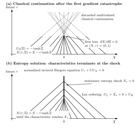
For $\partial_\tau U+\partial_X(U^2/2)=0$ with $U_0(X)=-\tanh X$, the characteristic map first loses invertibility at $(X,\tau)=(0,1)$. Panel (a) shows the discarded multivalued classical continuation; panel (b) shows the entropy solution, whose characteristics enter the stationary compressive shock $X_s=0$. Exact normalized characteristic geometry; selected characteristics only.

The crossed curves are not several physical velocities at one point; they announce the failure of the inviscid classical solution. With positive viscosity,

$$\partial_tu+u\partial_xu=\nu\partial_x^2u, \qquad \nu\gt0,$$

diffusion prevents literal gradient blow-up and resolves a layer whose thickness scales as $\nu/\Delta u$. The limit $\nu\to0^+$ selects the entropy weak solution. A molecular gas, plasma, or numerical scheme may have a different internal regularization, so Burgers flow explains the kinematics of steepening without claiming a universal microscopic shock profile.

Weak solutions and admissible shocks

Once a discontinuity forms, the conservative equation—not its expanded smooth form—is primary. Integrating across a moving discontinuity with speed $s$ yields the Rankine–Hugoniot condition

$$\boxed{ s[\mathbf U]=[\mathbf F], } \qquad [g]\equiv g_R-g_L.$$

For Burgers flow,

$$s=\frac{F(U_L)-F(U_R)}{U_L-U_R} =\frac{U_L+U_R}{2}.$$

The odd profile in the figure has $U_R=-U_L$, hence $s=0$. Moreover,

$$U_L\gt s\gt U_R,$$

so characteristics enter the shock from both sides. This compressive ordering is the scalar Lax condition.

Conservation alone does not select a unique weak solution. For a convex mathematical entropy $\eta(\mathbf U)$ with compatible entropy flux $q(\mathbf U)$, an admissible dissipative solution obeys

$$\partial_t\eta+\partial_xq\leq0$$

in the distributional sense. Thermodynamic entropy uses the opposite sign convention and increases through a physical compressive shock. Bressan derives Rankine–Hugoniot conditions and compares vanishing-viscosity, entropy, and Lax admissibility in Bressan 2026, §§2.1 and 2.3, printed pp. 11–20, then constructs elementary shock and rarefaction families in Bressan 2026, §§3.2–3.3, printed pp. 25–31.

The familiar equivalence among compression, a Lax inequality, convex-entropy dissipation, and vanishing viscosity is secure for a scalar convex flux and extends under specific strict-hyperbolicity and genuine-nonlinearity hypotheses. It is not a universal equivalence for every system or every regularization. Ideal MHD has degeneracies and compound waves; Hall, resistive, dispersive, or kinetic structure can admit non-Lax shocks. An admissibility rule must therefore be tied to the governing model.

Worked example: a gamma-law normal shock

Consider a steady planar, unmagnetized shock in its rest frame. Let $v\gt0$ be the normal velocity through the shock, let subscripts $1$ and $2$ denote upstream and downstream states, and define the specific enthalpy

$$h=e+\frac{p}{\rho}.$$

Mass, normal momentum, and total energy conservation give

$$\rho_1v_1=\rho_2v_2=j,$$ $$p_1+\rho_1v_1^2=p_2+\rho_2v_2^2,$$ $$h_1+\frac{v_1^2}{2} =h_2+\frac{v_2^2}{2}.$$

For a gamma-law gas with $\gamma\gt1$, choose the admissible compressive branch $M_1\gt1$. The point $M_1=1$ is the trivial no-jump limit; extending the nontrivial branch to $M_1\lt1$ would describe an entropy-decreasing expansion shock. On the compressive branch,

$$h=\frac{\gamma}{\gamma-1}\frac{p}{\rho}, \qquad c^2=\frac{\gamma p}{\rho}, \qquad M_1=\frac{v_1}{c_1}.$$

Eliminating $j$, $v_2$, and the downstream enthalpy gives

$$\boxed{ \frac{\rho_2}{\rho_1} =\frac{(\gamma+1)M_1^2} {(\gamma-1)M_1^2+2}, }$$ $$\boxed{ \frac{p_2}{p_1} =\frac{2\gamma M_1^2-(\gamma-1)} {\gamma+1}, \qquad M_2^2 =\frac{1+\frac{\gamma-1}{2}M_1^2} {\gamma M_1^2-\frac{\gamma-1}{2}}. }$$

For $\gamma=5/3$ and $M_1=3$,

$$\frac{\rho_2}{\rho_1}=3, \qquad \frac{p_2}{p_1}=11, \qquad M_2=\sqrt{\frac3{11}}\simeq0.522.$$

The upstream flow is supersonic and the downstream flow subsonic in the shock frame. The entropy change satisfies

$$\frac{\Delta s}{c_v} =\ln\left[ \frac{p_2/p_1}{(\rho_2/\rho_1)^\gamma} \right] =\ln\left(\frac{11}{3^{5/3}}\right)\gt0.$$

Thus the same calculation checks conservation, compressive ordering, and the physical second law. Tong derives these gas-dynamic jump relations and their entropy direction in Tong, current notes, §4.6, Eqs. (4.98)–(4.113), printed pp. 169–178.

Rayleigh–Taylor growth and its cutoff

An instability statement is incomplete until the equilibrium, boundaries, perturbation class, and retained physics are specified. For a clean example, put an inviscid incompressible fluid of density $\rho_+$ above one of density $\rho_-$, with gravity $g$ downward, no base flow, infinite depth, and surface tension $\Sigma$. Let the flat interface be perturbed by

$$\zeta(x,t)=\zeta_0e^{ikx+\gamma t}, \qquad k\gt0.$$

Irrotational perturbations have velocity potentials satisfying Laplace’s equation. Decay away from the interface fixes

$$\phi_+=A_+e^{-ky}e^{ikx+\gamma t}, \qquad \phi_-=A_-e^{ky}e^{ikx+\gamma t}.$$

The kinematic boundary condition $\partial_t\zeta=\partial_y\phi_\pm$ determines $A_\pm$. Linearized Bernoulli balance plus the capillary pressure jump then gives

$$\boxed{ \gamma^2 =A_{\rm t}gk-\frac{\Sigma k^3}{\rho_++\rho_-}, \qquad A_{\rm t}=\frac{\rho_+-\rho_-}{\rho_++\rho_-}. }$$

Here $A_{\rm t}$ is the Atwood number. When the heavier fluid is above, $A_{\rm t}\gt0$. If $\Sigma\gt0$, unstable modes satisfy

$$0\lt k\lt k_c, \qquad k_c=\sqrt{\frac{(\rho_+-\rho_-)g}{\Sigma}},$$

and the fastest idealized mode has

$$k_{\rm max}=\frac{k_c}{\sqrt3}.$$

If surface tension is omitted, this ideal discontinuous-interface model predicts ever faster growth as $k$ increases. That ultraviolet divergence is evidence that finite interface thickness, viscosity, diffusion, compressibility, or another small-scale effect has been omitted—not that arbitrarily short waves grow without physical limit. Tong develops the potential-flow derivation in Tong, current notes, §5.1, printed pp. 183–191.

Other instability diagnostics and their boundaries

• Kelvin–Helmholtz. A zero-thickness, unmagnetized vortex sheet with no restoring force is unstable to velocity shear in the simplest inviscid model. Density contrast, gravity, surface tension, finite shear thickness, compressibility, viscosity, and magnetic tension from a tangential field component parallel to the perturbation wavevector can alter the growth rate or introduce thresholds.
• Rayleigh’s inflection criterion. For inviscid incompressible parallel shear flow, an inflection point is a necessary condition for a normal-mode instability under the theorem’s hypotheses. It is not sufficient and is not a universal criterion for turbulence. Tong states the theorem and its limitations in §5.4, printed pp. 204–214.
• Ideal-MHD energy principle. For a static equilibrium, a self-adjoint ideal-MHD force operator, and admissible boundary conditions, finding a displacement with $\delta W\lt0$ proves linear instability. The test does not supply nonlinear saturation and does not transfer unchanged to equilibria with flow, resistivity, radiation, or kinetic closure. Murphy derives this variational criterion in Murphy 2016, Eqs. (23)–(41), printed slides 16–26.

All of these are early-time statements about a declared model. Later evolution may form shocks, current sheets, turbulence, or mixing layers and then require dissipation, kinetic physics, radiation, or a conservative numerical weak-solution method.

Waves and shocks in relativistic matter

This page uses nonrelativistic continuum and MHD equations. In compact-object flows, characteristic speeds must remain inside the light cone, conserved fluxes are built from covariant stress–energy and Maxwell equations, and shock conditions are evaluated relative to a spacetime hypersurface. The later Relativistic Magnetohydrodynamics and Plasmas chapter makes that replacement. The present Burgers calculation remains useful as a local model of nonlinear steepening, not as a derivation of a relativistic shock’s microphysics.

Exercises

Expansion instead of compression

For $u_0(x)=A\tanh(x/L)$ with $A,L\gt0$, determine whether forward-time Burgers characteristics intersect.

Solution

The derivative is

$$u_0'(\xi)=\frac{A}{L}\operatorname{sech}^2(\xi/L)\gt0.$$

Hence

$$\frac{\partial x}{\partial\xi} =1+t\,u_0'(\xi)\gt1$$

for every $t\gt0$. The characteristics spread and the smooth solution does not form a forward-time shock. The sign of the initial slope, not nonlinearity alone, distinguishes this rarefactive behavior from the decreasing profile in the figure.

A diatomic-gas normal shock

For $\gamma=7/5$ and upstream Mach number $M_1=2$, compute $\rho_2/\rho_1$, $p_2/p_1$, $T_2/T_1$, and $M_2$.

Solution

Substitution in the normal-shock formulas gives

$$\frac{\rho_2}{\rho_1}=\frac83, \qquad \frac{p_2}{p_1}=\frac92, \qquad M_2^2=\frac13.$$

Because $T\propto p/\rho$ for an ideal gas,

$$\frac{T_2}{T_1} =\frac{p_2/p_1}{\rho_2/\rho_1} =\frac{27}{16}, \qquad M_2=\frac1{\sqrt3}\simeq0.577.$$

The density, pressure, and temperature all rise, while the shock-frame Mach number falls below one.

References

• Bressan, Alberto. Lecture Notes on One Dimensional Hyperbolic Conservation Laws. Penn State University course notes (25 July 2026), §§1.1–1.5, 2.1, 2.3, and 3.2–3.3, printed pp. 1–8, 11–20, and 25–31. Official author PDF.
• Murphy, Nicholas A. “MHD Instabilities.” Harvard Astronomy 253 lecture notes (2016), Eqs. (23)–(41), printed slides 16–26. Official author PDF.
• Tong, David. Fluid Mechanics. University of Cambridge course notes (current online version), §§4.4.1, 4.6, 5.1, and 5.4, printed pp. 144–148, 169–178, 183–191, and 204–214. Official author PDF.