Kepler Orbits and Orbital Elements

A Kepler orbit is fixed by one position and one velocity at an epoch. Energy and angular momentum determine the conic’s size and shape; the remaining four data orient that conic in space and locate the body on it. The six classical orbital elements are therefore coordinates on initial-data space, not six new forces.

Required background. Classical and Variational Mechanics provides action principles, canonical variables, and mechanical conservation laws; Newtonian Gravity provides the gravitational potential, Poisson equation, and inverse-square force law. Helpful background. Calculus and Linear Algebra provides multivariable differentiation, linear maps, inner products, and basis changes; Ordinary Differential Equations provides initial-value problems, linearization, and asymptotic solution methods.

From the orbit equation to a conic

We describe relative motion in the potential per unit reduced mass

$$\Phi(r)=-\frac{\mathcal G}{r}, \qquad \mathcal G=G(m_1+m_2),$$

and use the specific angular momentum $\mathbf h=\mathbf r\times\mathbf v$ and specific energy $\varepsilon=v^2/2-\mathcal G/r$. This notation avoids confusing the gravitational parameter $\mathcal G$ with the binary’s reduced mass.

The replacement of a fixed-primary parameter by $G(m_1+m_2)$ follows from the exact two-body reduction in Tong 2013, §5.1.5, pp. 71–72, PDF. The Binet reduction below assumes $h\ne0$ and therefore excludes purely radial collision or ejection solutions, which must instead be treated directly with the radial energy equation.

To obtain an equation for the shape rather than its timing, put $u=1/r$ and choose the direction of increasing $\phi$ so that $h=r^2\dot\phi\gt0$. The chain rule gives

$$\dot r=-h\frac{du}{d\phi}, \qquad \ddot r=-h^2u^2\frac{d^2u}{d\phi^2}.$$

Substitute these into $\ddot r-r\dot\phi^2=-\mathcal G/r^2$ and divide by $-h^2u^2$. The result is Binet’s equation,

$$\frac{d^2u}{d\phi^2}+u=\frac{\mathcal G}{h^2}.$$

Choosing the polar axis through periapsis gives

$$r(\nu)=\frac{p}{1+e\cos\nu}, \qquad p=\frac{h^2}{\mathcal G},$$

where $\nu$ is the true anomaly, $p$ the semilatus rectum, and $e\ge0$ the eccentricity. Substituting this solution in the energy integral yields the invariant relation

$$e^2=1+\frac{2\varepsilon h^2}{\mathcal G^2}.$$

Thus, for nonradial motion, $\varepsilon\lt0$ gives $0\le e\lt1$ and an ellipse, $\varepsilon=0$ gives $e=1$ and a parabola, and $\varepsilon\gt0$ gives $e\gt1$ and a hyperbola. The classification follows from the conserved quantities, not from the appearance of a plotted arc. At $h=0$, even a negative-energy radial collision orbit has the degenerate value $e=1$, so the energy-only labels do not describe a regular conic.

For an ellipse, define the semimajor axis $a$ by

$$\varepsilon=-\frac{\mathcal G}{2a}, \qquad p=a(1-e^2), \qquad r_{\rm p}=a(1-e),\quad r_{\rm a}=a(1+e).$$

The corresponding hyperbolic convention often takes $a\lt0$, preserving $\varepsilon=-\mathcal G/(2a)$. Any quoted $a$ must therefore state its sign convention.

Period and anomaly variables

Area is swept at the constant rate $h/2$. Combining the ellipse area $\pi a^2\sqrt{1-e^2}$ with $h^2=\mathcal G a(1-e^2)$ gives

$$T=2\pi\sqrt{\frac{a^3}{\mathcal G}}, \qquad T^2=\frac{4\pi^2}{\mathcal G}a^3.$$

This is Kepler’s third law for relative motion with both masses retained. Replacing $m_1+m_2$ by only the larger mass is the test-particle approximation.

Time is most conveniently recovered with the eccentric anomaly $E$. It is the parameter in the Cartesian representation of the ellipse, with its occupied focus at the origin and periapsis along $+x$:

$$x=a(\cos E-e), \qquad y=a\sqrt{1-e^2}\sin E.$$

The circle before the $y$ direction is compressed has polar angle $E$ about the ellipse’s center; the body’s polar angle about the focus is the true anomaly $\nu$. Computing $r=\sqrt{x^2+y^2}$ and using constant swept area gives

$$r=a(1-e\cos E), \qquad M\equiv n(t-t_{\rm p})=E-e\sin E, \qquad n=\sqrt{\frac{\mathcal G}{a^3}}.$$

Indeed, $x\dot y-y\dot x=a^2\sqrt{1-e^2}(1-e\cos E)\dot E=h$, so $(1-e\cos E)\dot E=n$. Integrating from periapsis, where $E=0$, produces Kepler’s equation $E-e\sin E=n(t-t_{\rm p})$. It is transcendental but monotone because $1-e\cos E\gt0$ for $0\le e\lt1$, so a bracketed root finder is robust. The mean anomaly $M$ grows uniformly; neither $M$ nor $E$ is generally the geometric polar angle $\nu$.

The six classical elements

A nondegenerate bound orbit is commonly specified by

$$(a,e,i,\Omega,\omega,M_0),$$

at an epoch. Here $i$ and the longitude of ascending node $\Omega$ orient the orbital plane, $\omega$ locates periapsis within that plane, and $M_0$ locates the body along the orbit. The pair $(a,e)$ fixes size and shape.

The separation is easiest to see geometrically. In the figure, inspect first how $a$, $e$, and the true anomaly $\nu$ describe one in-plane ellipse, then how $\Omega$, $i$, and $\omega$ place that ellipse relative to a reference plane. Both planes contain the line of nodes. The ascending node is the crossing where the body moves toward positive reference height; $\omega$ is measured from that direction toward periapsis in the direction of orbital motion. The instantaneous $\nu$ plays the phase role that $M_0$ records at the chosen epoch.

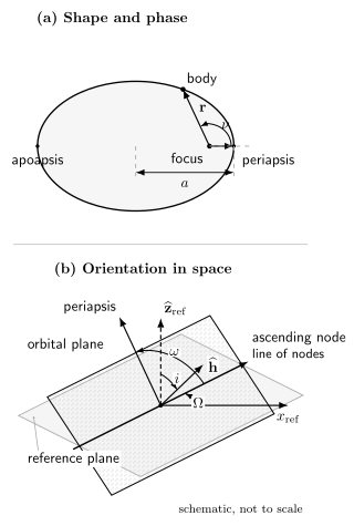
The six classical elements separate into size and shape $(a,e)$, orbital phase, and orientation $(\Omega,i,\omega)$. Panel (a) shows the ellipse and true anomaly; panel (b) projects both planes and their shared node line from one three-dimensional construction. The arrow along the node line points toward the ascending node; the angle arcs lie in their defining planes before projection. Schematic and not to scale.

These coordinates have singular cases. If $e=0$, periapsis is not distinguished and $\omega$ is undefined. If $i=0$ or $i=\pi$, the orbital and reference planes coincide, so there is no unique ascending node and $\Omega$ is undefined. The physical state is regular; only this element chart is singular. Vectorial elements, or an equinoctial chart chosen for the relevant inclination range, are preferable in numerical work near those limits.

The eccentricity vector makes the geometry coordinate-free within Euclidean space:

$$\mathbf e =\frac{\mathbf v\times\mathbf h}{\mathcal G}-\widehat{\mathbf r}, \qquad |\mathbf e|=e.$$

For $e\gt0$ it points toward periapsis. Direct differentiation with $\ddot{\mathbf r}=-\mathcal G\mathbf r/r^3$ verifies that $\dot{\mathbf e}=0$.

Checks and interpretation

• Dimensions give $[h^2/\mathcal G]=L$, as required for $p$, and $[a^3/\mathcal G]=T^2$.
• For $e=0$, $r=a=p$, $v^2=\mathcal G/a$, and the period reduces to circumference divided by circular speed.
• At fixed $a$, increasing $e$ changes periapsis and apoapsis but not the period. This special degeneracy belongs to the inverse-square law.
• A fitted osculating element set describes the Kepler conic tangent to a perturbed trajectory at one epoch. It is not a promise that the real trajectory repeats; see JPL Solar System Dynamics, “Orbital Elements” (accessed 2026).

The conic equation, energy–semimajor-axis relation, and period law are derived from the same conserved quantities in Tong 2013, §§4.3–4.3.2, pp. 55–62, PDF. The eccentric-anomaly time-of-flight relation and the elliptic, parabolic, and hyperbolic energy branches are collected in Peraire and Widnall 2008, Lecture L16, Eqs. (1)–(11), pp. 1–4, PDF.

Transfer task

A bound orbit is observed at periapsis $r_{\mathrm p}$ with purely transverse speed $v_{\mathrm p}$. Determine $e$ without first solving for the trajectory.

Solution

At periapsis, $h=r_{\mathrm p}v_{\mathrm p}$ and

$$\varepsilon=\frac{v_{\mathrm p}^2}{2}-\frac{\mathcal G}{r_{\mathrm p}}.$$

Insert these in the invariant eccentricity relation:

$$e^2 =1+\frac{2\varepsilon h^2}{\mathcal G^2} =\left(\frac{r_{\mathrm p}v_{\mathrm p}^2}{\mathcal G}-1\right)^2.$$

For periapsis rather than apoapsis, $v_{\mathrm p}\ge\sqrt{\mathcal G/r_{\mathrm p}}$, so

$$e=\frac{r_{\mathrm p}v_{\mathrm p}^2}{\mathcal G}-1.$$

Continue to The Newtonian Two-Body Problem to recover the two barycentric trajectories and the system’s total energy.

References

• Jet Propulsion Laboratory Solar System Dynamics. “Description of Orbits and Ephemerides.” “Orbital Elements”, accessed 2026.
• Peraire, Jaime, and Sheila Widnall. “Central Force Motion: Orbits.” MIT OpenCourseWare 16.07 Dynamics, Lecture L16, Fall 2008, version 1.1. Eqs. (1)–(11), pp. 1–4, PDF.
• Tong, David. Dynamics and Relativity. University of Cambridge lecture notes, Lent 2013. §§4.3–4.3.2, pp. 55–62; §5.1.5, pp. 71–72, PDF.