Area and Volume Operators

A spin network makes spatial geometry measurable through flux, not through a metric operator at a point. After a surface is partitioned into small cells, the flux in each cell acts by an $SU(2)$ generator on every transverse edge. Taking the square root of the quadratic Casimir gives a discrete area contribution. This is an exact statement about kinematical geometry in the Ashtekar–Lewandowski representation; it is not, by itself, a spectrum of a fully relational Dirac observable.

Required background. Variational and Symplectic Geometry supplies canonical brackets and regulated observables; Frames, Tetrads, and Spinors supplies triads and internal $SU(2)$ indices.

Helpful background. Flat-Spacetime Quantum Field Theory supplies operator quantization; Einstein Equations supplies the geometry to recover; Quantum Information supplies tensor-product and angular-momentum language; and Quantum Gravity supplies the distinction between kinematics and physical prediction.

Area as a regulated flux norm

Let $S$ be an oriented, piecewise semianalytic two-surface in a spatial slice, and let $n_a$ denote its coordinate normal density. In real Ashtekar–Barbero variables, with $\ell_{\mathrm P}^2=G$, its classical area is

$$A(S)=\int_S d^2\sigma\, \sqrt{E_i(S,\sigma)E^i(S,\sigma)}, \qquad E_i(S,\sigma)=n_aE^a_i.$$

Partition $S$ into cells $S_I$ small enough that each contains at most one simple, transverse puncture of a chosen graph. The Riemann sum

$$A(S)=\lim_{N\to\infty}\sum_I \sqrt{E_i(S_I)E^i(S_I)}$$

is well suited to quantization because each integrated flux already belongs to the holonomy–flux algebra. On an edge $e$ in spin-$j_e$ representation, a transverse flux acts as

$$\widehat E_i(S_I)\,D^{(j_e)}(h_e) =\pm 8\pi\gamma G\, D^{(j_e)}(h_{e_1})J_i^{(j_e)}D^{(j_e)}(h_{e_2}),$$

where the sign follows the oriented intersection together with the holonomy and generator convention. It disappears after contracting internal indices, and $J_iJ^i=j(j+1)\mathbf1$. Thus, for punctures away from graph vertices,

$$\begin{aligned} \widehat A(S)\lvert\Gamma,\{j_e\},\{\iota_v\}\rangle &=A_{\Gamma,S}\lvert\Gamma,\{j_e\},\{\iota_v\}\rangle,\\ A_{\Gamma,S} &=8\pi\lvert\gamma\rvert G\sum_{p\in S\cap\Gamma} \sqrt{j_p(j_p+1)}. \end{aligned}$$

This standard spectrum and the more general vertex formula are derived in Ashtekar and Lewandowski 1997, §§III–IV. At a vertex lying in $S$, upward, downward, and tangent edge generators must first be combined; simply counting edges can then give the wrong eigenvalue.

Why the eigenvalues are discrete

The discreteness has two ingredients. Cylindrical states depend on finitely many holonomies, so the regulated operator reduces to finitely many angular-momentum operators. Compactness of $SU(2)$ then makes their Casimir spectrum discrete. It is not a coordinate lattice effect: the regulator cells disappear, while the graph intersections remain as diffeomorphism-covariant data.

Three checks fix the interpretation. First, $j=0$ and a tangent edge contribute zero, as a flux through $S$ should. Second, one transverse $j=\tfrac12$ puncture gives

$$A_{1/2}=8\pi\lvert\gamma\rvert G\sqrt{\frac34} =4\pi\sqrt3\,\lvert\gamma\rvert G.$$

With $[G]=L^2$ and dimensionless $j$ and $\gamma$, this has area dimension. Third, at large $j$,

$$\sqrt{j(j+1)}=j+\frac12+O(j^{-1}),$$

so the relative spacing tends to zero even though the exact kinematical spectrum remains discrete. This is one route by which coarse semiclassical areas can look continuous.

Volume lives at vertices

For a region $R$,

$$V(R)=\int_R d^3x\sqrt{\left|\frac1{3!} \epsilon_{abc}\epsilon^{ijk}E^a_iE^b_jE^c_k\right|}.$$

Triangulate $R$ and replace the three triads by fluxes through three small faces. After removing the regulator, the operator is a sum over graph vertices,

$$\widehat V(R)=(8\pi\lvert\gamma\rvert G)^{3/2} \sum_{v\in R}\sqrt{\lvert\widehat q_v\rvert}, \qquad \widehat q_v=C\!\sum_{e_I,e_J,e_K\ni v} \epsilon(e_I,e_J,e_K)\epsilon^{ijk} J_i^{I}J_j^{J}J_k^{K},$$

where $C$ depends on the precisely declared regularization and $\epsilon(e_I,e_J,e_K)$ records the orientation of the three edge tangents. The operator acts on the finite-dimensional intertwiner space at $v$, so its eigenvalues are again discrete. Coplanar triples have zero orientation factor; a gauge-invariant trivalent vertex also has zero volume, while sufficiently noncoplanar vertices of valence four or more can carry volume. The construction and the regularization choices are developed in Ashtekar and Lewandowski 1998, §§II–V.

An intertwiner is an invariant way to combine the edge angular momenta at a vertex into total spin zero. It records information about how the incident face fluxes fit together. Edges therefore supply area labels, while their coupling at a vertex supplies the additional information needed for volume. A four-valent vertex can still have zero volume for a coplanar embedding or an appropriate intertwiner; valence four is permission for nonzero volume, not a guarantee.

The prefactor has dimension $(L^2)^{3/2}=L^3$, as required. Unlike the simple-puncture area formula, volume eigenvalues depend on intertwiners and on diagonalizing $\widehat q_v$; valence labels alone do not determine them. The displayed $C$ keeps the regularization choice visible, so this formula does not assign a numerical volume eigenvalue until that choice is fixed.

The sketch separates the data used by the two operators. Follow the transverse edges through the surface, then compare their puncture labels with the additional vertex data in the lower panel.

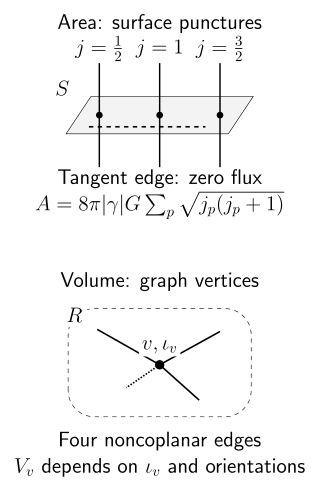
Area reads edge spins at simple transverse punctures; a tangent edge contributes no flux. Volume acts at vertices and also reads the intertwiner and edge orientations. The dotted lower edge indicates depth in this perspective sketch, not a missing edge. Noncoplanarity alone does not fix a nonzero eigenvalue. Kinematical schematic, not a spatial lattice or a physical minimum-length claim.

Kinematical result, physical question

Area and volume commute with the Gauss constraint when their internal indices are contracted, and their diffeomorphism-covariant definitions survive graph refinement. They generally do not commute with the Hamiltonian constraint. A coordinate-specified surface or region therefore does not yet define a physical measurement. One must identify it relationally—for example, as a matter-defined surface—and construct the corresponding Dirac observable. The resulting physical spectrum need not follow merely from the kinematical spectrum. Ashtekar and Lewandowski 2004, §§IV.4–IV.6 and VI emphasize both the exact kinematical results and this dynamical boundary.

The Barbero–Immirzi parameter $\gamma$ supplies a further warning: the eigenvalue scale depends on a quantization parameter not fixed by classical vacuum general relativity. Discreteness is robust within the representation and operator definitions stated here; the numerical gap and its observable status require additional physics.

Exercises

A surface is punctured transversely by three edges carrying $j=\tfrac12$, $1$, and $\tfrac32$, with no puncture at a vertex. Find the area eigenvalue and check its large-spin and zero-spin limits.

Solution

The simple-puncture formula gives

$$A=8\pi\lvert\gamma\rvert G\left( \frac{\sqrt3}{2}+\sqrt2+\frac{\sqrt{15}}2 \right).$$

Every term is nonnegative and the orientation signs have canceled inside the Casimir. Replacing any label by $j=0$ removes that puncture. Replacing all three by a common large $j$ gives $A=24\pi\lvert\gamma\rvert G[j+\tfrac12+O(j^{-1})]$, whose fractional level spacing is $O(j^{-1})$. The calculation would not apply unchanged if the punctures coincided at a surface vertex, because the incident generators must then be coupled before taking the square root.

References

• Ashtekar, Abhay, and Jerzy Lewandowski. “Background Independent Quantum Gravity: A Status Report.” Classical and Quantum Gravity 21 (2004): R53–R152. Open manuscript.
• Ashtekar, Abhay, and Jerzy Lewandowski. “Quantum Theory of Geometry I: Area Operators.” Classical and Quantum Gravity 14 (1997): A55–A82. DOI.
• Ashtekar, Abhay, and Jerzy Lewandowski. “Quantum Theory of Geometry II: Volume Operators.” Advances in Theoretical and Mathematical Physics 1 (1998): 388–429. Open manuscript.