Evaporating Black-Hole Diagram Families

There is no single established conformal diagram for an evaporating four-dimensional black hole. Hawking radiation on a prescribed collapse background, a self-consistent mean geometry during slow mass loss, and a complete spacetime with an endpoint are three different levels of claim. The controlled large-hole calculation can stop before the complete future is known; an event horizon and an endpoint diagram cannot be read off from that partial history.

Helpful background. Hawking Flux, Backreaction, and Evaporation Dynamics supplies the physical hierarchy, while Black Hole Formed by Collapse fixes the one-ended classical comparison. An Event Horizon Is Not Every Black-Hole Boundary distinguishes global and quasi-local horizons. This page uses schematic four-dimensional spherical radial quotients in the sense of Frauendiener 2004, §§ 1–2; the two-dimensional CGHS and RST models appear only as model-specific comparisons.

From Hawking flux to a causal geometry

The logical ladder has five rungs:

1. choose a quantum state on a prescribed collapse geometry;
2. compute a renormalized stress tensor and outgoing luminosity;
3. solve for the geometry’s response;
4. verify that curvature, adiabatic error, stress fluctuations, and omitted operators remain controlled; and
5. add a future continuation only if further physics specifies one.

Hawking’s mode calculation supplies the prescribed-background state-and-mode analysis and the asymptotic-flux part of the second rung, but not a complete renormalized stress tensor on an evolving geometry, a backreacted metric, or an endpoint Hawking 1975, § 2, pp. 204–211, and § 4, pp. 218–219. A mean geometry would instead have to satisfy an equation of the form

$$G_{ab}+\Lambda g_{ab}+H^{\mathrm{ren}}_{ab} =8\pi G_{\mathrm{ren}} \langle T_{ab}\rangle_{\omega,\mathrm{ren}}, \qquad \frac{dM_{\mathrm B}}{du}=-L_\infty.$$

Here $H^{\mathrm{ren}}_{ab}$ collects the retained local gravitational counterterms, $\omega$ names the state, $M_{\mathrm B}$ is Bondi mass, and positive luminosity $L_\infty$ decreases it. The equation is effective: a small mean source is not enough if stress fluctuations or higher-curvature terms become important. The mean-field, stochastic-response, and large-$N$ validity questions are separated in Hu and Verdaguer 2008, §§ 2–5.

Let $\Sigma_*$ denote the last spacelike surface on which all declared control tests pass. It is a calculation cutoff—not automatically a singularity, endpoint, matching surface, or conformal boundary. The adiabatic evaporation approximation and the current self-consistency criteria explain how such a cutoff arises.

A shrinking marginal tube is not an event horizon

For a chosen asymptotically flat end $E$, the global black-hole region and future event horizon are

$$\mathcal B_E=\mathcal M\setminus J^-(\mathscr I_E^+), \qquad \mathcal H_E^+=\partial J^-(\mathscr I_E^+).$$

Both definitions require the completed spacetime and its future null infinity. Booth’s horizon comparison makes this teleological dependence explicit Booth 2005, §§ 2.1–2.3, pp. 1075–1081. By contrast, a future outer marginal surface can be specified on a slice by

$$\theta_{(\ell)}=0, \qquad \theta_{(n)}\lt0, \qquad \mathcal L_n\theta_{(\ell)}\lt0,$$

for outward and inward future null normals $\ell^a$ and $n^a$. Its world tube is foliation-sensitive and need not be null. Hayward’s trapping-horizon laws state their classical energy-condition hypotheses explicitly Hayward 1994, §§ III and V, pp. 4–8; Hawking evaporation violates the relevant null-energy sign, so the classical signature conclusion cannot simply be imported.

The ingoing Vaidya proxy gives a direct check:

$$ds^2=-\left(1-\frac{2Gm(v)}{r}\right)dv^2 +2\,dv\,dr+r^2d\Omega^2, \qquad T_{vv}=\frac{\dot m}{4\pi r^2}.$$

On the marginal tube $r=2Gm(v)$, a tangent is $\xi^a=(\partial_v)^a+2G\dot m(\partial_r)^a$, so

$$g_{ab}\xi^a\xi^b=4G\dot m.$$

With signature $(-,+,+,+)$, evaporation has $\dot m\lt0$ and this tube is timelike. That calculation neither locates an event horizon nor supplies the full Unruh-state stress tensor: one ingoing Vaidya patch does not simultaneously model the outgoing flux at $\mathscr I^+$. The precise flux and area interpretation is developed in Negative Energy and Horizon Shrinkage.

Read the assumption map

Inspect where each panel stops being a calculation and starts being an added future. The two lower completion panels share the same controlled data on $\Sigma_*$; the picture deliberately supplies no rule that selects between them. This family is representative rather than exhaustive.

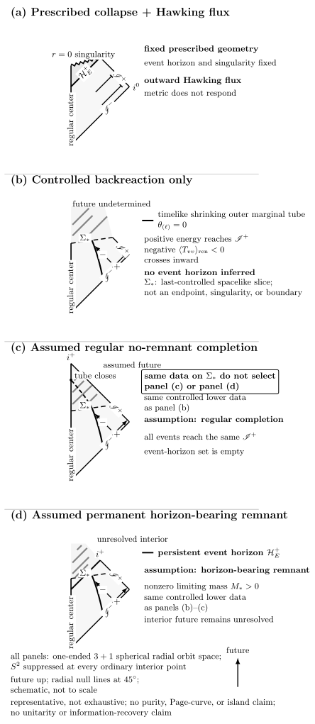
Four sketches separate levels of claim rather than asserting one evaporation spacetime. Panel (a) places Hawking flux on a prescribed collapse background and does not evolve the geometry. Panel (b) shows only a controlled backreaction segment: positive flux reaches future null infinity, negative renormalized energy crosses a shrinking outer marginal tube, and the prediction stops at the last-controlled surface $\Sigma_*$. Panels (c) and (d) append, respectively, an explicitly assumed regular no-remnant future and an explicitly assumed permanent horizon-bearing remnant; their common lower data do not select between them. An event horizon may be identified only after a complete future has been supplied. Causal incidence alone determines neither purity, a Page curve, islands, nor an information-recovery channel. Future points upward; all four-dimensional spherical radial sketches are schematic and not to scale.

Sketch or continuation	What is supplied	What does not follow
Prescribed-background flux	Quantum fields on a fixed one-ended collapse geometry	Metric shrinkage, disappearance, or an endpoint
Controlled backreaction to $\Sigma_*$	Mean geometry, flux balance, and a timelike outer marginal tube in the displayed proxy	A complete future or a global event-horizon verdict
Regular no-remnant future	An assumed regular continuation in which the marginal tube closes and every event reaches the same $\mathscr I^+$	A derivation of the required stress tensor, stability, or unitarity
Permanent horizon-bearing remnant	An assumed $M_*\gt0$ future with persistent causal inaccessibility	Information capacity, genericity, or long-term stability
Horizonless remnant	A timelike compact-object world tube after the trapped region disappears	A black-hole region or event horizon merely from the word “remnant”
Singular, thunderbolt, or last-ray future	A specified terminal boundary and its causal character	Selection by the large-hole approximation
Bounce or new asymptotic region	Additional dynamics and global topology	Absence of an event horizon relative to the original $\mathscr I^+$
Two-dimensional RST comparisons	A controlled breakdown result or an exactly solvable modified model with chosen endpoint data	The four-dimensional causal diagram

Hayward’s regular construction is an explicit example of the third row: it assumes a metric and flux profile whose inner and outer trapping horizons join around a compact trapped region, leaving a regular future Hayward 2006, Eqs. (1)–(23), Figs. 3–5, pp. 3–4. Giddings’ explicitly speculative massive-remnant diagram instead illustrates the horizonless-remnant row: the horizon meets the proposed core, leaving a large information-bearing object rather than a permanent black-hole event horizon or a generic Planck-sized endpoint Giddings 1992, §§ 1–4 and Figs. 2–3. Neither construction is selected by the common lower history, and neither validates the horizon-bearing panel.

The lower-dimensional literature sharpens the same boundary without fixing four-dimensional gravity. The early RST analysis of the one-loop CGHS equations finds a receding timelike apparent horizon but loses control before evaporation completes Russo, Susskind, and Thorlacius 1992, §§ II–IV. The later counterterm-modified RST model is exactly solvable until its apparent horizon meets the singularity; continuing it requires boundary data, and the authors’ chosen matching produces a small negative-energy “thunderpop” Russo, Susskind, and Thorlacius 1992, §§ 1–4. Hawking and Stewart compare naked and thunderbolt alternatives but explicitly retain their model and higher-derivative limitations Hawking and Stewart 1993, §§ 1 and 3–5. Two-Dimensional Backreaction Models develops these distinctions; Endpoint Regimes and Remnant Questions compares the stable assumption classes.

Causal topology does not encode quantum information

A conformal diagram records causal incidence. It contains no density matrix, subsystem factorization, entanglement entropy, quantum extremal surface, replica saddle, Page curve, or recovery map. Two quantum states can live on the same causal spacetime, and an island calculation can change an entropy prescription without changing the drawn Lorentzian causal geometry. Conversely, a regular future with no event horizon establishes causal accessibility only under its declared completion; it does not prove pure-state evolution.

The information alternatives and their carrier assumptions belong to Information Loss, Remnants, and Long-Lived Interiors, not to the line topology of this figure. For mutable evidence judgments, use the dated assessments of self-consistent black-hole evaporation and evaporation endpoints and remnants.

Common pitfalls

Calling $\Sigma_*$ the endpoint. It marks where the retained approximation ceases to justify further evolution. A physical endpoint requires additional equations, boundary data, or microscopic dynamics.

Equating the shrinking tube with the event horizon. The tube is defined quasi-locally by an expansion; the event horizon is defined globally from the completed future. They can differ in location, signature, and even existence.

Importing a two-dimensional graph into four dimensions. CGHS/RST field content, counterterms, state prescription, and boundary conditions are part of their results. Exact solvability does not erase dimensional dependence.

Reading information flow from an arrow. The flux arrows denote renormalized energy balance, not local particle-pair worldlines or a channel carrying a specified quantum state.

Evidence boundary

Checked 2026-08-24, the controlled evidence supports fixed-background Hawking flux, slow large-hole mass loss, local backreaction models, and exact lower-dimensional laboratories. It does not select a universal neutral four-dimensional endpoint. The representative family should be revisited if a reproducible self-consistent four-dimensional solution controls the evolution through $\Sigma_*$, or if a proposed completion acquires a fully specified state, renormalized source, constraints, error budget, and global future.

References

• Booth, Ivan. “Black-Hole Boundaries.” Canadian Journal of Physics 83 (2005), 1073–1099, §§ 2–5. DOI: 10.1139/p05-063.
• Frauendiener, Jörg. “Conformal Infinity.” Living Reviews in Relativity 7 (2004), article 1, §§ 1–2. DOI: 10.12942/lrr-2004-1.
• Giddings, Steven B. “Black Holes and Massive Remnants.” Physical Review D 46 (1992), 1347–1352, §§ 1–4. DOI: 10.1103/PhysRevD.46.1347.
• Hawking, Stephen W. “Particle Creation by Black Holes.” Communications in Mathematical Physics 43 (1975), 199–220, with erratum 46 (1976), 206. DOI: 10.1007/BF02345020.
• Hawking, Stephen W., and John M. Stewart. “Naked and Thunderbolt Singularities in Black Hole Evaporation.” Nuclear Physics B 400 (1993), 393–415. DOI: 10.1016/0550-3213(93)90410-Q.
• Hayward, Sean A. “Formation and Evaporation of Nonsingular Black Holes.” Physical Review Letters 96 (2006), 031103. DOI: 10.1103/PhysRevLett.96.031103.
• Hayward, Sean A. “General Laws of Black-Hole Dynamics.” Physical Review D 49 (1994), 6467–6474. DOI: 10.1103/PhysRevD.49.6467.
• Hu, Bei-Lok, and Enric Verdaguer. “Stochastic Gravity: Theory and Applications.” Living Reviews in Relativity 11 (2008), article 3. DOI: 10.12942/lrr-2008-3.
• Russo, Jorge G., Leonard Susskind, and Lárus Thorlacius. “Black Hole Evaporation in 1+1 Dimensions.” Physics Letters B 292 (1992), 13–18. DOI: 10.1016/0370-2693(92)90601-Y.
• Russo, Jorge G., Leonard Susskind, and Lárus Thorlacius. “End Point of Hawking Radiation.” Physical Review D 46 (1992), 3444–3449. DOI: 10.1103/PhysRevD.46.3444.