Reissner–Nordström Conformal Diagrams

Charge divides the exact Reissner–Nordström family into three different causal graphs. Two simple roots give the infinitely repeating subextremal extension; one double root gives a distinct extremal extension; no real root leaves a naked timelike singularity. These are statements about four-dimensional, asymptotically flat Einstein–Maxwell electrovac with $\Lambda=0$, not about which diagram is produced by regular collapse or survives perturbations.

Helpful background. Reissner–Nordström Horizons and Extensions constructs the horizon-regular charts and maximal extensions used here. Causality and Global Structure supplies event horizons, Cauchy horizons, and conformal boundaries.

Three regimes from one radial polynomial

Use signature $(-,+,+,+)$, set $c=1$, and use Gaussian electromagnetic units. For mass $M$, electric charge $Q_e$, magnetic charge $Q_m$, and areal radius $r$,

$$m=GM,\qquad q^2=GQ^2=G\left(Q_e^2+Q_m^2\right),\qquad M\gt0,\quad r\gt0.$$

The mechanics records use rationalized rather than Gaussian charge. Their complete Maxwell normalization map leaves the geometric parameter $q^2$ and first-law work term unchanged.

The static form is

$$ds^2=-f(r)\,dt^2+\frac{dr^2}{f(r)}+r^2d\Omega_2^2, \qquad f(r)=1-\frac{2m}{r}+\frac{q^2}{r^2} =\frac{(r-r_+)(r-r_-)}{r^2},$$

where

$$r_\pm=m\pm\sqrt{m^2-q^2}.$$

The root and sign tests give the whole regime key. Bičák develops the charged exact solution and its causal structures in Bičák 2000, § 3, printed pp. 31–41, PDF.

Regime	Roots and sign of $f$	Exact causal graph
$0\lt q^2\lt m^2$	Two simple positive roots; $f\gt0$ for $r\gt r_+$ and $0\lt r\lt r_-$, while $f\lt0$ for $r_-\lt r\lt r_+$	Repeating subextremal chain with outer Killing horizons—whose future branches are event horizons—and inner Cauchy horizons
$q^2=m^2$	One double root $r_+=r_-=m$; $f=(1-m/r)^2\ge0$	Repeating extremal graph with a degenerate horizon, but no trapped band or bifurcation sphere
$q^2\gt m^2$	No real root; $f\gt0$ throughout $r\gt0$	One static asymptotic domain with no horizon or repeated block

The strict lower bound in the first row matters: $q=0$ is Schwarzschild, whose spacelike singularity and four-region block are not obtained by simply erasing the inner-horizon labels from a charged diagram.

The three causal graphs

The figure suppresses every symmetry two-sphere and draws radial null directions at $45^\circ$. Future points upward. Solid heavy diagonals mark outer or degenerate Killing-horizon components; the future outer branches are event horizons relative to the displayed asymptotic ends. Dashed diagonals mark Cauchy-horizon components, jagged lines mark curvature-singular boundaries, and dotted continuation marks mean that the analytic graph repeats rather than ends. Conformal compactification preserves causal incidence, not metric distance or area; see Frauendiener 2004, §§ 1–2.

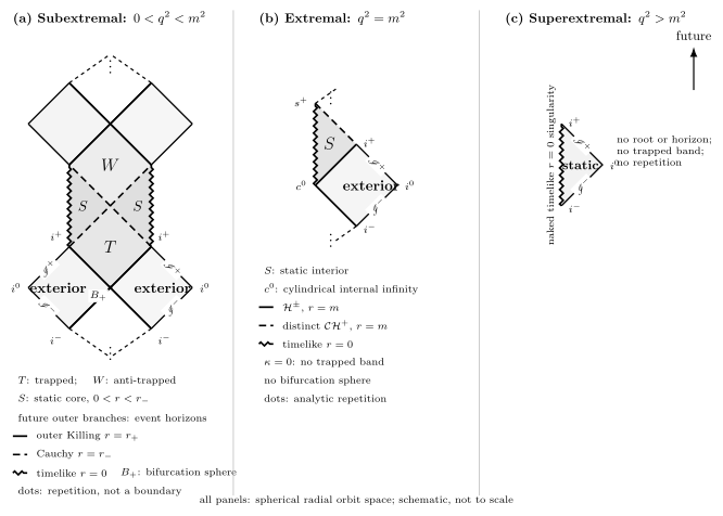
Charge separates the exact Reissner–Nordström family into three causal graphs: an infinitely repeating subextremal extension with outer and inner horizons, a distinct extremal extension with a degenerate horizon and no bifurcation sphere, and a horizonless superextremal spacetime with a naked timelike singularity. Future points upward; each spherical radial diagram is schematic and not to scale.

Diagram element	Geometric meaning
Exterior diamond	One asymptotically flat static end, with $\mathscr I^-$, $\mathscr I^+$, $i^-$, $i^+$, and $i^0$
$r=r_+$ in the strict subextremal panel	Outer Killing-horizon branches; relative to the displayed asymptotic ends, the future branches are event horizons
$r=r_-$ in the strict subextremal panel	Inner null branches that bound a globally hyperbolic region and act as Cauchy horizons in the exact extension
$r=m$ in the extremal panel	Degenerate null surface with zero surface gravity; the event- and Cauchy-horizon components shown are globally distinct even though their areal radius agrees
Jagged $r=0$ line	Timelike curvature-singular boundary, not conformal infinity
Continuation marks	Matching edges of neighboring analytic blocks; they are not physical boundaries or traversability claims

Subextremal analytic chain

For $0\lt q^2\lt m^2$, a future-directed crossing of a future $r=r_+$ branch enters a trapped region where $r$ is timelike; the past branch instead borders the time-reversed anti-trapped region. Beyond an $r=r_-$ branch lies another static region bounded by timelike $r=0$ singularities. Horizon-regular patches can then be glued through further inner and outer branches, producing an infinite analytic chain in both time directions rather than a single Schwarzschild-like block. Graves and Brill give the two-root patching and global gluing in Graves and Brill 1960, Eqs. (21)–(27), § IV, and Fig. 3, printed pp. 1510–1512.

The smooth Cauchy horizons belong to the exact stationary solution. Calling them smooth here does not say that generic radiation can cross them with the same regularity.

Extremal is not a collapsed subextremal diagram

At $q^2=m^2$, the double root has surface gravity $\kappa=0$ and $f$ never becomes negative. The trapped band therefore disappears. More importantly, the global limit is nonuniform: the standard extremal extension has no outer-horizon bifurcation sphere. Its event-horizon and future Cauchy-horizon components are distinct null components at the common radius $r=m$, joined through a graph with a cylindrical internal infinity and analytic repetition.

Carter constructs this exceptional maximal extension directly in Carter 1966, printed pp. 423–424. A modern exact-background diagram with the same event horizon, Cauchy horizon, internal infinity, timelike singularity, and repetition appears in Angelopoulos, Kehle, and Unger 2026, § 2.2, printed pp. 20–22, especially Fig. 7 on p. 20. Their nonlinear theorem has additional spherical Einstein–Maxwell–scalar and codimension-one hypotheses; this page uses only their exact-background topology.

Superextremal naked singularity

For $q^2\gt m^2$, $f$ stays positive, so the static domain runs from the one asymptotic end down to $r=0$. No zero of $f$ supplies a Killing horizon, event horizon, Cauchy horizon, trapped band, or seam into another analytic block. The timelike singularity is therefore in the causal past of future null infinity: it is naked in this exact spacetime. That statement neither proves that regular initial data form this solution nor settles weak or strong cosmic censorship.

Curvature and limit checks

The Kretschmann scalar is

$$R_{\mu\nu\rho\sigma}R^{\mu\nu\rho\sigma} =\frac{48m^2}{r^6}-\frac{96mq^2}{r^7}+\frac{56q^4}{r^8}.$$

It is finite at every positive horizon radius and diverges as $r\to0$. The horizon-regular charts developed in Reissner–Nordström Horizons and Extensions show that the roots extend as regular null hypersurfaces; finiteness of this one scalar alone would not prove that result. The invariant instead independently detects each jagged $r=0$ line as a curvature singularity.

Two topology limits require care. As $q\to0$ at fixed exterior data, $r_-\to0$ and the entire inner structure collapses into the central singular region; the neutral causal graph must be replaced by the maximally extended Schwarzschild diagram. As $q^2\to m^2$ from below, the two roots merge algebraically, but the extremal diagram is obtained from its own global extension, not by squeezing the two horizon lines together.

Exact background versus dynamical interior

This record establishes no $C^0$, $C^1$, or $C^2$ stability result, no mass-inflation endpoint, no traversability, no formation mechanism, and no censorship conclusion. For those questions, use Reissner–Nordström and Kerr Interiors, the dated Inner Horizons and Mass Inflation record, and Near-Extremal and Extremal Stability.

References

• Angelopoulos, Yannis, Christoph Kehle, and Ryan Unger. “Nonlinear Stability of Extremal Reissner–Nordström Black Holes in Spherical Symmetry.” Forum of Mathematics, Pi 14 (2026), e3, § 2.2, pp. 20–22. DOI: 10.1017/fmp.2025.10017.
• Bičák, Jiří. “The Role of Exact Solutions of Einstein’s Equations in the Developments of General Relativity and Astrophysics: Selected Themes.” In Einstein’s Field Equations and Their Physical Implications, edited by Bernd G. Schmidt, 1–126. Lecture Notes in Physics 540. Springer (2000), § 3, printed pp. 31–41. Open PDF.
• Carter, Brandon. “The Complete Analytic Extension of the Reissner–Nordström Metric in the Special Case $e^2=m^2$.” Physics Letters 21 (1966), 423–424. DOI: 10.1016/0031-9163(66)90515-4.
• Frauendiener, Jörg. “Conformal Infinity.” Living Reviews in Relativity 7 (2004), article 1, §§ 1–2. DOI: 10.12942/lrr-2004-1.
• Graves, John C., and Dieter R. Brill. “Oscillatory Character of Reissner–Nordström Metric for an Ideal Charged Wormhole.” Physical Review 120 (1960), 1507–1513. DOI: 10.1103/PhysRev.120.1507.