Maximally Extended Schwarzschild Diagram

The maximally extended Schwarzschild solution contains two asymptotically flat exteriors, a future black-hole interior, and a past white-hole interior. Its conformal diagram records the radial causal incidence of those four Kruskal regions. It represents the eternal analytic vacuum solution with mass $M\gt 0$, not the spacetime of a body formed by collapse.

Helpful background. Causality and Global Structure supplies causal relations, horizons, conformal boundaries, and the distinction between local cones and global causal claims.

Four-region causal structure

Let $r_s=2GM$ and choose Kruskal null coordinates in the right exterior so that

$$-UV=\left(\frac{r}{r_s}-1\right)e^{r/r_s}.$$

The horizons are the regular null surfaces $U=0$ and $V=0$; their intersection $U=V=0$ is the bifurcation two-sphere. The future and past $r=0$ boundaries satisfy $UV=1$ and are spacelike curvature singularities. Convention, domain, and four-sector checks are given by Reall 2013, §§ 12.5–12.6, printed pp. 141–148, PDF and Bičák 2000, § 2, printed pp. 19–30, PDF.

The diagram below is schematic: radial null lines are drawn at $45^\circ$, but coordinate distances and displayed areas have no metric meaning. Inspect the two crossed horizon branches and the different characters of the null infinities and jagged singular boundaries.

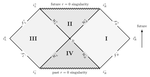
The maximally extended eternal Schwarzschild solution has right and left exteriors (I and III), a future black-hole region (II), and a past white-hole region (IV). Future points upward; solid diagonal boundaries are null, and jagged horizontal boundaries are the spacelike $r=0$ curvature singularities. The diagram is schematic and not to scale; each interior point represents a symmetry two-sphere.

Region and boundary key

Label	Geometric meaning	Causal role
I	Right asymptotically flat exterior, $U\lt 0\lt V$	Static observers run from $i^-_{R}$ to $i^+_{R}$; escaping light reaches $\mathscr I^+_{R}$
II	Black-hole interior, $U\gt 0$, $V\gt 0$	Areal radius decreases toward the future; every future-inextendible causal curve approaches the future $r=0$ singularity
III	Left asymptotically flat exterior, $V\lt 0\lt U$	A second asymptotic end, causally distinct from Region I
IV	White-hole interior, $U\lt 0$, $V\lt 0$	Future-directed causal curves emerge from the past $r=0$ singularity
$\mathcal H^+_{R,L}$	Two components of the future event horizon	Future null boundaries of the causal pasts of the corresponding $\mathscr I^+$ components
$\mathcal H^-_{R,L}$	Two components of the past horizon	Past null boundaries associated with the white-hole region
$B$	Bifurcation two-sphere, $U=V=0$	Intersection of all four horizon branches; fixed set of the Schwarzschild Killing flow
$\mathscr I^\pm_{R,L}$	Future and past null infinity for each asymptotic end	Ideal endpoints of escaping and incoming null curves
$i^0_{R,L}$	Spatial infinity of each end	Ideal endpoint of asymptotically spatial directions
$i^\pm_{R,L}$	Future and past timelike infinity of each end	Ideal endpoints of asymptotically stationary timelike curves
Future and past $r=0$	Spacelike curvature-singular boundaries	Curvature divergence forbids a $C^2$ Lorentzian extension; these are not conformal infinity

No future-directed causal curve travels from Region I to Region III. A spacelike slice can connect the two ends through the bifurcation sphere, but the Einstein–Rosen bridge is not causally traversable.

Eternal extension versus collapse

Time reversal supplies the white-hole region and past singularity; completing the analytic continuation through both horizon branches supplies the second exterior. None is forced by the late-time exterior metric. In the standard one-ended spherical-collapse model, a regular material center replaces the past white-hole geometry and there is no second asymptotic end; the future event horizon and black-hole region remain, but their global past is different. Reall makes this distinction explicit in Reall 2013, §§ 12.5–12.6, printed pp. 141–148, PDF.

Checks and limitations

The horizon is regular because the Kruskal metric coefficient is finite and nonzero at $UV=0$. In contrast,

$$R_{\mu\nu\rho\sigma}R^{\mu\nu\rho\sigma} =\frac{48G^2M^2}{r^6}$$

is finite at $r=r_s$ and diverges as $r\to0$. This independently distinguishes the crossed null horizons from the jagged singular boundaries.

The drawing preserves radial causal order, not affine length or four-dimensional scale. Its open $\mathscr I^\pm$ segments are null conformal boundaries; $i^0$ and $i^\pm$ are limiting ideal points with different regularity. For the general treatment of the construction and its causal-boundary meaning, see Conformal Completion, Causal Boundaries, and Penrose Diagrams. The detailed construction and boundary-classification tests are given in Constructing Penrose Diagrams, with the conformal-boundary conditions reviewed in Frauendiener 2004, §§ 1.1–1.3.

References

• Bičák, Jiří. “The Role of Exact Solutions of Einstein’s Equations in the Developments of General Relativity and Astrophysics: Selected Themes.” In Einstein’s Field Equations and Their Physical Implications, edited by Bernd G. Schmidt, 1–126. Lecture Notes in Physics 540. Springer (2000), § 2, printed pp. 19–30. Open PDF.
• Frauendiener, Jörg. “Conformal Infinity.” Living Reviews in Relativity 7, article 1 (2004). DOI: 10.12942/lrr-2004-1.
• Reall, Harvey S. General Relativity. Cambridge Part III lecture notes (2013), §§ 12.5–12.6, printed pp. 141–148. PDF.