Exponential Maps and Normal Neighborhoods

The exponential map turns an initial tangent vector into the endpoint, at affine parameter one, of its geodesic. Smooth dependence on initial data and the inverse function theorem make this map a local diffeomorphism near the zero vector. That local theorem produces normal coordinates and convex normal neighborhoods; it does not make the exponential map globally injective, surjective, or even globally defined.

Required background. Affine Connections and Covariant Derivatives supplies the general connection and covariant-derivative framework; Affine and Variational Geodesics supplies the affine geodesic equation and its initial-value interpretation. The Riemann Curvature Tensor fixes the curvature convention used when the differential of the exponential map is analyzed through Jacobi fields.

Helpful background. Calculus and Linear Algebra for Relativity supplies multivariable differentiation and linear maps; the needed ODE existence and inverse-function results are stated on this page. Presymplectic Potentials and Currents is an advanced field-space continuation, not a prerequisite for the exponential map.

Definition and natural domain

For $p\in M$ and $v\in T_pM$, let $\gamma_v$ be the maximally extended affinely parametrized geodesic satisfying

$$\gamma_v(0)=p, \qquad \dot\gamma_v(0)=v.$$

Whenever $1$ lies in its parameter domain, define

$$\exp_p(v)=\gamma_v(1).$$

The natural domain $\mathcal D_p\subset T_pM$ is open and star-shaped about $0$: if $v\in\mathcal D_p$, then $tv$ remains admissible for $0\le t\le1$, and $\gamma_v(t)=\exp_p(tv)$. On an incomplete manifold, $\mathcal D_p$ need not be all of $T_pM$.

In flat affine coordinates, $\exp_p(v)=p+v$. On a round sphere $S^n_a\subset\mathbb R^{n+1}$ with $a\gt0$ and $n\ge2$,

$$\exp_p(v)= \cos\!\left(\frac{\lvert v\rvert}{a}\right)p +a\sin\!\left(\frac{\lvert v\rvert}{a}\right) \frac{v}{\lvert v\rvert},$$

with the continuous value $p$ at $v=0$. Every vector of length $\pi a$ maps to the antipode $-p$, exhibiting global noninjectivity.

The local diffeomorphism theorem

At $v=0$, the differential is the identity:

$$(d\exp_p)_0=\operatorname{id}_{T_pM}.$$

To see it, take $w\in T_pM$ and the curve $s\mapsto sw$ in $T_pM$. Then

$$(d\exp_p)_0w =\left.\frac{d}{ds}\right|_{s=0}\exp_p(sw) =\left.\frac{d}{ds}\right|_{s=0}\gamma_w(s)=w.$$

The inverse function theorem therefore supplies neighborhoods $U\ni0$ and $V\ni p$ for which $\exp_p:U\to V$ is a diffeomorphism. Taking the components of its inverse in a basis of $T_pM$ gives normal coordinates. The radial lines in $T_pM$ map to geodesics through $p$. For a Levi–Civita connection, choose that initial basis orthonormal; then at $p$,

$$g_{\mu\nu}=\eta_{\mu\nu}, \qquad \Gamma^\rho{}_{\mu\nu}=0, \qquad \partial_\lambda g_{\mu\nu}=0.$$

Curvature generally prevents the second metric derivatives from vanishing. The construction and proof appear in Tong 2019, §3.3, pp. 118–129.

Normal and convex normal neighborhoods

A normal neighborhood of $p$ is an open set reached diffeomorphically from a star-shaped neighborhood of $0\in T_pM$. Every point in it is joined to $p$ by a unique radial geodesic lying in that neighborhood. A convex normal neighborhood is stronger: any two of its points are joined by a unique geodesic contained entirely inside it. Such neighborhoods exist around every point of a smooth pseudo-Riemannian manifold after shrinking sufficiently.

This uniqueness is local. It does not say that no second geodesic leaves the neighborhood and returns, or that the selected segment is globally optimal. In Riemannian signature, Gauss’s lemma shows sufficiently short radial geodesics minimize length. In Lorentzian signature, causal character changes the extremal statement: short timelike segments locally maximize proper time, spacelike behavior differs, and null length is identically zero. The local differential-geometric theorem itself does not rely on a positive-definite distance.

Failure of global injectivity

The sphere gives the clean test. On the open tangent ball $\lvert v\rvert\lt\pi a$, $\exp_p$ is a diffeomorphism onto the sphere with its antipode removed. At $\lvert v\rvert=\pi a$, every direction reaches $-p$. The differential loses rank in transverse directions, and infinitely many great semicircles join the endpoints. The antipode is both conjugate and a cut point here, but those notions need not coincide on a general manifold.

The figure pairs this geometric collapse with the exact transverse Jacobi amplitude. Inspect how all angular directions meet at $-p$, where the amplitude vanishes, while each great-circle geodesic continues beyond the meeting point.

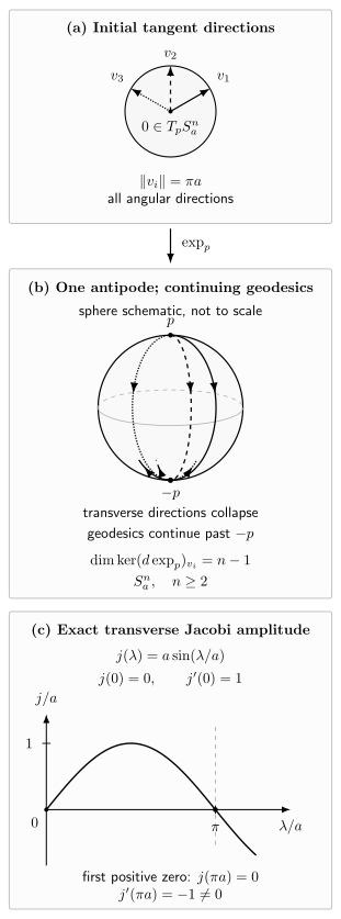
On $S^n_a$ with $n\ge2$, every tangent direction of length $\pi a$ at $p$ reaches the antipode, where transverse Jacobi fields vanish and $(d\exp_p)_v$ loses rank. The great-circle geodesics nevertheless continue beyond that point, so conjugacy and cut behavior do not imply incompleteness. Schematic sphere with the exact amplitude $j(\lambda)=a\sin(\lambda/a)$ for unit initial transverse relative velocity.

There are two other distinct global failures. On an incomplete manifold, some $\gamma_v(1)$ may not exist, so the exponential map has a restricted domain. On a flat but topologically identified manifold, the map may be defined everywhere and locally nonsingular while failing global injectivity through multiple winding geodesics. Local curvature, conjugacy, topology, and completeness are separate mechanisms.

Normal coordinates are centered data, not a single preferred chart for the whole manifold. Changing the base point changes the exponential map and the chart. At the center, vanishing connection coefficients remove first-order inertial effects, while the Taylor expansion begins to reveal curvature at quadratic order. Along radial geodesics the coordinate components are linear in affine parameter, but arbitrary coordinate lines need not be geodesics.

A convex normal neighborhood is especially useful because it defines a unique separation vector $\exp_x^{-1}(y)$ for every ordered pair of points inside it. Bitensors and world functions use exactly this local uniqueness. Once a cut or conjugate structure is crossed, that inverse becomes multivalued or singular; formulas based on a unique connecting geodesic must then be restricted rather than extended by notation alone.

The theorem and the construction of normal neighborhoods are treated in Sternberg 2003, Chapter VI, pp. 125–131. Physical claims about free fall or global causal connection lie outside this local geometric result.

Exercises

Use the sphere formula to show that the differential of $\exp_p$ is singular at every $v$ with $\lvert v\rvert=\pi a$.

Solution

For $n\ge2$, vary $v$ through vectors of fixed length $\pi a$ but changing direction. The endpoint remains $\cos(\pi)p+a\sin(\pi)v/\lvert v\rvert=-p$. Hence every infinitesimal angular variation is mapped to zero. These transverse directions form an $(n-1)$-dimensional kernel of $(d\exp_p)_v$, so the differential is singular.

The restriction $n\ge2$ matters. On the circle $S^1_a$, there is no transverse direction: the exponential map wraps a line around the circle and is everywhere a local diffeomorphism. The antipode is still a cut point, because two shortest arcs meet there, but it is not conjugate.

References

• Sternberg, Shlomo. Semi-Riemann Geometry and General Relativity. Course notes, Harvard University, 2003. PDF.
• Tong, David. General Relativity. University of Cambridge Part III Mathematical Tripos lecture notes, 2019. PDF.