Optical Tensors and Sachs Evolution

The optical tensor turns geodesic deviation into the first-order evolution of a narrow beam of null rays. Its trace controls cross-sectional area, its symmetric trace-free part controls image distortion, and its antisymmetric part controls twist. The Sachs equations are the screen-projected Riccati equation for this tensor; they are exact geometric statements before any field equation or lens model is chosen.

The first-order and second-order descriptions serve different purposes. The optical tensor displays instantaneous rates and decomposes them cleanly, while the Jacobi map remains the safer object at a focal point and carries the endpoint data needed for a beam. Moving between them is legitimate only where that map is invertible.

Required background. The Riemann Curvature Tensor fixes the sign of the curvature tidal map; Affine and Variational Geodesics supplies null geodesics, affine parameters, and the variation setup; Jacobi Fields and Geodesic Deviation derives the deviation equation and initial-data map from which the screen Jacobi matrix is built. Helpful background. Calculus and Linear Algebra for Relativity supplies matrix differential equations, determinants, and trace-free decomposition; Frames, Coframes, and Anholonomy supplies a transported screen basis.

The Jacobi map of a light beam

Let $k^\mu$ be an affinely parametrized null tangent in four spacetime dimensions. Choose an orthonormal screen basis $E_A^\mu$, $A=1,2$, parallel transported along a fiducial ray, along with a parallel-transported auxiliary null vector. A transverse connecting field has screen components $\xi^A$. Two solutions associated with the chosen family can be organized into a Jacobi matrix $D^A{}_B$:

$$\xi^A(\lambda)=D^A{}_B(\lambda)\,\alpha^B,$$

where $\alpha^B$ labels the family. For rays launched from one vertex, these labels can be initial angular directions, with $D(\lambda_0)=0$ and $\dot D(\lambda_0)=I$ after fixing the affine scale and screen units. For a beam launched from a finite cross-section, different initial data apply. The Jacobi matrix is defined even at a caustic; only its inverse requires nonzero determinant. Define the screen tidal matrix by

$$\mathcal T_{AB} =R_{\mu\alpha\nu\beta} E_A^\mu k^\alpha E_B^\nu k^\beta.$$

With the site curvature convention, the screen Jacobi equation is

$$\ddot D=-\mathcal T D.$$

The trace satisfies $\operatorname{tr}\mathcal T=R_{\mu\nu}k^\mu k^\nu$. Its trace-free part records anisotropic curvature on the screen. This split is geometric; interpreting either part through matter or a gravitational field equation lies beyond the present construction.

From deviation to a Riccati equation

Where $D$ is invertible, set

$$\mathcal B=\dot D D^{-1}.$$

Differentiation gives

$$\dot{\mathcal B} =\ddot D D^{-1}-\dot D D^{-1}\dot D D^{-1} =-\mathcal T-\mathcal B^2.$$

This matrix Sachs equation is equivalent to the projected evolution of $\nabla_\nu k_\mu$. It also makes its domain transparent: $\mathcal B$ ceases to be represented by this formula when $\det D=0$, although $D$ itself can remain a smooth solution through that parameter value.

Write

$$\mathcal B_{AB} =\frac{\theta}{2}\delta_{AB} +\sigma_{AB} +\omega_{AB}.$$

Taking the trace yields the affine null Raychaudhuri identity

$$\dot\theta =-\frac12\theta^2 -\sigma_{AB}\sigma^{AB} +\omega_{AB}\omega^{AB} -R_{\mu\nu}k^\mu k^\nu.$$

In two screen dimensions, the square of a symmetric trace-free matrix and the square of an antisymmetric matrix are both multiples of the identity; their anticommutator vanishes. The other two projections therefore reduce to

$$\dot\sigma_{AB}=-\theta\sigma_{AB}-\mathcal T_{\langle AB\rangle}, \qquad \dot\omega_{AB}=-\theta\omega_{AB},$$

where $\mathcal T_{\langle AB\rangle}=\mathcal T_{AB}-\tfrac12\delta_{AB}\operatorname{tr}\mathcal T$. Thus trace-free tidal curvature drives shear, while initially zero twist remains zero wherever the optical system is regular. These simplified equations are special to a two-dimensional screen; the full matrix equation applies in higher dimensions. Perlick derives the Jacobi tensor, optical scalars, and image-distortion map in Perlick 2004, §§2.3–2.5.

Area and image shape

An infinitesimal beam area is proportional to

$$\mathcal A=\left|\det D\right|.$$

Jacobi’s determinant formula immediately gives

$$\frac{\dot{\mathcal A}}{\mathcal A} =\operatorname{tr}(\dot D D^{-1}) =\theta.$$

Thus expansion is the logarithmic area rate. The image of an initial unit circle is governed by the polar decomposition

$$D=RU, \qquad U=\left(D^{\mathsf T}D\right)^{1/2}.$$

Here $R$ is orthogonal and the eigenvalues $s_1,s_2$ of the positive polar factor $U$ are the singular values of $D$. Order them as $s_1\ge s_2\ge0$; away from a caustic, $s_2\gt0$. They are the semiaxis lengths of the image ellipse, so $s_1s_2=|\det D|$ gives its area scale and $s_1/s_2$ gives its axis ratio. Unlike the eigenvalues of the additive symmetric part of $D$, these quantities are unchanged by rotations of the initial or final screen bases. Shear changes the ratio of principal stretches. With both screen orientations fixed, $R$ is a rotation when $\det D\gt0$ and reverses orientation when $\det D\lt0$; an odd parity change across a caustic can therefore change the type of $R$. The instantaneous twist is instead the antisymmetric part of $\mathcal B$. Where $D$ is invertible the polar factorization is unique; at rank loss, $U$ and its singular values remain well defined although $R$ need not be unique. These are local properties of an infinitesimal bundle. Turning them into angular-diameter distance, magnification, or a finite-image observable requires endpoint normalization and an observer setup.

The figure follows one initial screen label through an anisotropically stretched section and then to rank loss. Inspect the ellipse semiaxes before the caustic and the precise inverse-dependent quantity that ceases to exist when one stretch vanishes.

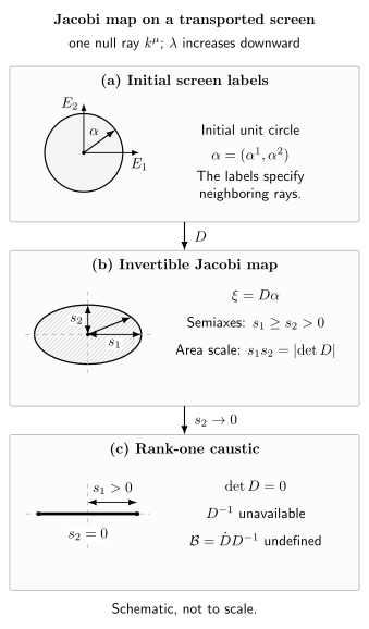
The Jacobi map carries initial transverse labels to screen separations. Before the caustic its singular values are the beam ellipse semiaxes and $\mathcal B=\dot D D^{-1}$; when one stretch vanishes, $D$ loses rank and the inverse-based optical tensor fails although the Jacobi equation may remain regular. Schematic and not to scale.

For generators of a null hypersurface the twist vanishes. Then a screen basis can be rotated to display the two real shear components, but their individual values depend on that basis; the norm $\sigma_{AB}\sigma^{AB}$ does not. A null boost rescales $\mathcal B$ and changes the affine parameter, so the normalization of $k^\mu$ must be held fixed when comparing optical scalars.

Radial Minkowski verification

For outgoing radial rays in four-dimensional Minkowski spacetime, choose an affine parameter with $r=\lambda$ up to an additive constant. Two small angular separations produce physical screen separations proportional to $r$, so

$$D=rI, \qquad \mathcal B=\frac1r I.$$

It follows that

$$\theta=\frac2r, \qquad \sigma_{AB}=0, \qquad \omega_{AB}=0.$$

Since $\mathcal T=0$, the matrix equation gives $\dot{\mathcal B}=-\mathcal B^2=-I/r^2$. Its trace is $\dot\theta=-2/r^2=-\theta^2/2$, exactly as required. This simultaneously checks the sign of the Riccati equation, the factor of two in the screen trace, and the area law $\mathcal A\propto r^2$.

An initially elliptical beam in flat spacetime can have a nonzero shear during part of its propagation if its Jacobi initial data are anisotropic. Curvature is a driver of optical evolution, not the only possible source of nontrivial initial optical data.

Common pitfalls

The optical tensor is singular at a caustic, not necessarily the Jacobi map. The inverse $D^{-1}$ fails when $\det D=0$. Continue with the second-order Jacobi equation rather than declaring the spacetime singular.

Screen components require transport choices. A rotating screen basis can introduce apparent rotation of components. State how the basis is propagated and distinguish that choice from invariant twist.

A geometric beam is not yet an observed image. Endpoint conditions, source and observer velocities, and normalization turn the Jacobi map into distance and distortion observables. The local Sachs equations alone do not fix them.

Exercises

Suppose a twist-free, curvature-free beam has

$$D(\lambda)= \begin{pmatrix} \lambda & 0\\ 0 & \lambda+c \end{pmatrix},$$

on an interval where both factors are positive. Find its expansion and shear eigenvalues.

Solution

One obtains

$$\mathcal B=\dot D D^{-1} =\operatorname{diag}\left(\frac1\lambda,\frac1{\lambda+c}\right).$$

Therefore

$$\theta=\frac1\lambda+\frac1{\lambda+c},$$

and the shear eigenvalues are

$$\pm\frac12\left(\frac1\lambda-\frac1{\lambda+c}\right).$$

The area is $\mathcal A=\lambda(\lambda+c)$, whose logarithmic derivative is precisely $\theta$. The example shows how anisotropic initial data can produce shear even when the curvature tidal matrix vanishes.

References

• Perlick, Volker. “Gravitational Lensing from a Spacetime Perspective.” Living Reviews in Relativity 7, 9 (2004). doi:10.12942/lrr-2004-9.