Dynamical Tides and Mode Resonances

A tide must be evolved as an internal degree of freedom when the applied field changes on a timescale comparable with a coupled stellar mode, when a resonance is crossed, or when the response retains memory of earlier forcing. The minimal model is a driven quadrupolar oscillator coupled to the orbit. It reproduces the static Love response far below resonance, remains finite through a controlled resonance crossing, and accounts for energy stored in the body. Damping is a separate ingredient: a frequency-dependent conservative response can exist with no dissipation, while damped response transfers coherent mechanical energy into heat, outgoing radiation, or other unresolved degrees of freedom.

Helpful background. The Einstein Equation supplies the covariant curvature coupling; Weak Metric Perturbations and Gauge Freedom supplies perturbative mode variables; Presymplectic Potentials and Currents supplies the variational energy exchange; Relativistic Matter and Compact Objects supplies stellar mode spectra; Relativistic Two-Body Dynamics supplies the evolving orbit; and Black-Hole Perturbation Theory supplies retarded boundary conditions and quasinormal response.

A quadrupole as a driven mode

For one nonrotating body’s dominant electric quadrupole, take

$$L_Q =\frac{1}{4\lambda_0\omega_f^2} \left(\dot Q^{ij}\dot Q_{ij} -\omega_f^2Q^{ij}Q_{ij}\right) -\frac12Q^{ij}\mathcal E_{ij}.$$

The tensors are symmetric, tracefree, and spatial in a nonrotating body frame. Dots denote proper-time derivatives; at the Newtonian order used in this oscillator they coincide with orbital coordinate-time derivatives. Assume $\omega_f^2\gt0$ and $\lambda_0\gt0$, so the free mode is stable and has positive energy. These constants are respectively the mode frequency and its contribution to the zero-frequency deformability. Variation gives

$$\ddot Q_{ij}+\omega_f^2Q_{ij} =-\lambda_0\omega_f^2\mathcal E_{ij}.$$

This normalization is chosen so that the limit $\omega_f\rightarrow\infty$ gives $Q_{ij}=-\lambda_0\mathcal E_{ij}$, exactly the adiabatic convention. Steinhoff, Hinderer, Buonanno, and Taracchini give this Newtonian oscillator and its covariant worldline extension in Steinhoff et al. 2016, §§ I A–I C, Eqs. (1.1)–(1.8).

Phenomenological linear damping changes the equation to

$$\ddot Q_{ij}+2\gamma_f\dot Q_{ij}+\omega_f^2Q_{ij} =-\lambda_0\omega_f^2\mathcal E_{ij}.$$

With the Fourier convention $e^{-i\omega\tau}$,

$$Q_{ij}(\omega) =-\lambda(\omega)\mathcal E_{ij}(\omega), \qquad \lambda(\omega) =\frac{\lambda_0\omega_f^2} {\omega_f^2-\omega^2-2i\gamma_f\omega}.$$

The real part describes elastic storage and dispersive frequency dependence. The imaginary part describes mechanical loss for $\gamma_f\gt0$. The poles are $\omega=-i\gamma_f\pm\sqrt{\omega_f^2-\gamma_f^2}$, in the lower half-plane for a stable damped mode. Setting $\gamma_f=0$ does not restore an instantaneous tide: the retarded limiting prescription and the mode’s free oscillations remain. An undamped monochromatic force applied exactly at resonance grows secularly; finiteness through a swept resonance is a different statement.

Even an undamped mode has a distributional imaginary part when the retarded prescription is kept:

$$\operatorname{Im}\lambda_{\rm ret}(\omega) \xrightarrow{\gamma_f\to0^+} \frac{\pi\lambda_0\omega_f}{2} \left[\delta(\omega-\omega_f)-\delta(\omega+\omega_f)\right].$$

This represents resonant transfer into the coherent mode, not entropy production. Away from its poles the undamped susceptibility is real; at a pole, forcing history and the stored mode energy must be retained. The steady-state absorption formula cannot be interpreted as a finite constant heating rate for an exactly undamped resonant oscillator.

The figure compares the real and imaginary parts with the static value. Inspect the low-frequency limit first, then the sign change and enhanced imaginary response near $\omega_f$. For $x=\omega/\omega_f$ and $\eta=\gamma_f/\omega_f$, the plotted quantities are

$$\frac{\operatorname{Re}\lambda}{\lambda_0} =\frac{1-x^2}{(1-x^2)^2+4\eta^2x^2}, \qquad \frac{\operatorname{Im}\lambda}{\lambda_0} =\frac{2\eta x}{(1-x^2)^2+4\eta^2x^2}.$$

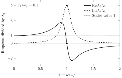
Quantitative steady response of one damped mode, normalized by its static deformability, for $\gamma_f/\omega_f=0.1$. At $\omega=\omega_f$, the real part vanishes and the imaginary part equals $5\lambda_0$; the dotted horizontal line is the static approximation. The damping ratio is chosen to make both curves visible, not fitted to a star. These are monochromatic steady responses, not the time evolution through a swept resonance.

An actual star has many modes. In a linear, nonrotating model its retarded response can be organized schematically as

$$\lambda_{\rm ret}(\omega) =\lambda_{\rm contact}(\omega) +\sum_\alpha \frac{\lambda_\alpha\omega_\alpha^2} {\omega_\alpha^2-\omega^2-2i\gamma_\alpha\omega}.$$

The residue $\lambda_\alpha$ contains the mode overlap with the tidal field. A local contact term is needed if the retained modes do not span the entire response. This is important in reduced models: fitting $\lambda_0$ and then adding an oscillator with the same zero-frequency contribution double counts the static deformability. The completeness and residual-contact issue are stated explicitly in Steinhoff et al. 2016, § II A, Eqs. (2.1)–(2.2).

Adiabatic expansion and its failure

Away from a pole and with negligible damping,

$$\lambda(\omega) =\lambda_0 \left[ 1+\frac{\omega^2}{\omega_f^2} +O\!\left(\frac{\omega^4}{\omega_f^4}\right) \right].$$

The first term is the static Love response. The next terms are conservative dynamical-tide corrections and correspond to higher time-derivative operators if the mode is integrated out. That derivative expansion is controlled only while $|\omega|/\omega_f\ll1$. It cannot be analytically continued through the pole by retaining more terms.

For a circular nonrotating binary, decompose the tide into STF spherical components,

$$\mathcal E_{ij}(\tau) =\sum_{m=-2}^{2}\mathcal E_m(\tau) \mathcal Y^{2m}_{ij}e^{-im\Phi(\tau)}.$$

The $m=\pm2$ components dominate the Newtonian quadrupolar forcing, and resonance occurs when $|m|\Omega\simeq\omega_f$. Eccentric motion supplies a larger set of harmonics $n\Omega_r+m\Omega_\phi$; precession and spin shift the body-frame frequency further. It is therefore unsafe to use “orbital frequency below the mode frequency” as the sole criterion without identifying the actual harmonic and frame.

Near a monotonic crossing, define the detuning

$$\Delta(\tau)=\omega_f-\omega_{\rm tide}(\tau).$$

The quasi-stationary amplitude proportional to $1/\Delta$ fails inside a resonance layer of duration and frequency width

$$t_{\rm res}\sim|\dot\omega_{\rm tide}|^{-1/2}, \qquad \delta\omega_{\rm res}\sim|\dot\omega_{\rm tide}|^{1/2}.$$

For an underdamped mode, the causal solution makes the history explicit:

$$\begin{aligned} Q_{ij}(\tau)={}&Q^{\rm hom}_{ij}(\tau)\\ &-\frac{\lambda_0\omega_f^2}{\omega_d} \int_{\tau_0}^{\tau}e^{-\gamma_f(\tau-\tau')} \sin[\omega_d(\tau-\tau')]\mathcal E_{ij}(\tau')\,d\tau', \end{aligned} \qquad \omega_d=\sqrt{\omega_f^2-\gamma_f^2}.$$

The homogeneous solution carries the initial mode displacement and velocity. For weak damping and a slow monotonic frequency sweep, expanding the forcing phase to quadratic order near the crossing turns this integral into a Fresnel integral. It remains finite over the crossing and leaves a free oscillation afterward. Thus no single-valued function of instantaneous separation captures the complete response. The resonance-layer scaling above requires $|\dot\omega_{\rm tide}|\ll\omega_f^2$ and slowly varying mode properties and forcing amplitude. Hinderer et al. construct the corresponding uniformly finite approximation in Hinderer et al. 2016, Eqs. (1)–(2).

Three timescales govern the crossing:

$$t_{\rm mode}=\omega_f^{-1}, \qquad t_{\rm res}=|\dot\omega_{\rm tide}|^{-1/2}, \qquad t_{\rm damp}=\gamma_f^{-1}.$$

If $t_{\rm damp}\gg t_{\rm res}$, the mode crosses resonance coherently and stores energy after the passage. If $t_{\rm damp}\ll t_{\rm res}$, a near-steady dissipative response may be appropriate. Neither limit follows merely from the value of the static Love number.

Energy transfer and orbital backreaction

For $\gamma_f=0$, the oscillator energy in our normalization is

$$E_Q =\frac{1}{4\lambda_0\omega_f^2} \left(\dot Q^{ij}\dot Q_{ij} +\omega_f^2Q^{ij}Q_{ij}\right).$$

Using the equation of motion,

$$\dot E_Q =-\frac12\mathcal E_{ij}\dot Q^{ij}.$$

The interaction energy is essential here. If $E_{\rm orb}^{(0)}$ excludes the tide, then $V_{\rm int}=Q^{ij}\mathcal E_{ij}/2$ and the orbital force give

$$\dot E_{\rm orb}^{(0)}=-\frac12Q^{ij}\dot{\mathcal E}_{ij}, \qquad \frac{d}{d\tau}\left(E_{\rm orb}^{(0)}+V_{\rm int}+E_Q\right)=0.$$

The two isolated work terms are not negatives of each other until the interaction energy is included. A conservative resonance redistributes energy and angular momentum within this complete system. With damping,

$$\dot E_Q =-\frac12\mathcal E_{ij}\dot Q^{ij} -\frac{\gamma_f}{\lambda_0\omega_f^2} \dot Q^{ij}\dot Q_{ij}.$$

The last term is mechanical energy lost by the resolved mode; a complete material model identifies where it goes, such as heat or radiation. In this explicit-mode description, the orbit supplies the tidal work while damping removes energy from $E_Q$. One must not subtract both the driving work and the same eventual dissipated energy as independent orbital losses. An alternative description may integrate out the mode and use a causal effective orbital force, but it must then account for the mode’s energy storage through that response.

The mode also carries angular momentum. Its canonical momentum is $P^{ij}=\dot Q^{ij}/(2\lambda_0\omega_f^2)$, so rotational invariance gives

$$(S_Q)_i=2\epsilon_{ijk}Q^{j\ell}P^k{}_\ell =\frac{\epsilon_{ijk}Q^{j\ell}\dot Q^k{}_\ell} {\lambda_0\omega_f^2}.$$

This contribution enters the relativistic Hamiltonian and the balance of angular momentum. The covariant constraints, tidal spin, and Legendre transformation are developed in Steinhoff et al. 2016, § II, especially Eqs. (2.4)–(2.31).

Radiation reaction now has two roles. It sweeps the forcing frequency through resonance, and the induced multipole contributes directly to emitted gravitational radiation. A consistent waveform evolves the orbital variables and $Q_{ij}$ together, includes their combined radiative multipoles, and distinguishes radiation to infinity from internal damping. The resonance phase shift depends on the mode frequency, overlap, sweep rate, damping, and initial mode state; it is not determined by $\lambda_0$ alone.

Effective resummations and validity tests

An efficient circular-orbit model may define

$$\lambda_{\rm eff}(\tau) =-\frac{\mathcal E_{ij}Q^{ij}} {\mathcal E_{kl}\mathcal E^{kl}}$$

and replace a static Love coefficient in an effective-one-body potential by $\lambda_{\rm eff}$. This can summarize the enhancement before resonance and is useful in waveform construction. Steinhoff et al. define this contraction and derive an EOB implementation in Steinhoff et al. 2016, Eq. (1.2) and § VI; Hinderer et al. compare a related effective-tide model with numerical-relativity calculations in Hinderer et al. 2016, Eqs. (3)–(6).

An effective coefficient is not automatically a material property. It can depend on orbital history, harmonic content, initial data, and the resummation map. Any proposed replacement should pass four checks:

1. it tends to $\lambda_0$ as $\omega_{\rm tide}/\omega_f\to0$;
2. its pole position and residue agree with the resolved oscillator;
3. it remains finite under the intended resonance-crossing prescription;
4. it does not count the same static contribution in both a contact operator and an explicit mode.

The linear mode model itself has boundaries. It assumes $|Q|/(mR^2)\ll1$, a background star that changes slowly compared with the mode, and a separation large enough for a worldline multipole expansion. Nonlinear mode coupling, mass shedding, shocks, contact, or disruption require additional physics. Close numerical agreement for one equation of state and mass ratio is evidence within that calibration region, not a proof of universal behavior.

Exercises

1. Recover the static tide. Expand the undamped response through $O(\omega^2)$ and translate it into the time domain.

Solution

For $|\omega|\lt \omega_f$,

$$\lambda(\omega) =\frac{\lambda_0}{1-\omega^2/\omega_f^2} =\lambda_0 \left(1+\frac{\omega^2}{\omega_f^2}+\cdots\right).$$

Since multiplication by $\omega^2$ corresponds to $-\partial_\tau^2$ with the $e^{-i\omega\tau}$ convention,

$$Q_{ij} =-\lambda_0\mathcal E_{ij} +\frac{\lambda_0}{\omega_f^2} \ddot{\mathcal E}_{ij} +O(\partial_\tau^4).$$

The first term is adiabatic response; the second is its leading conservative retardation correction. The series fails at the pole.

2. Check oscillator energy balance. Derive $\dot E_Q$ for nonzero $\gamma_f$.

Solution

Differentiate $E_Q$:

$$\dot E_Q =\frac{\dot Q^{ij}} {2\lambda_0\omega_f^2} \left(\ddot Q_{ij}+\omega_f^2Q_{ij}\right).$$

The damped equation replaces the parentheses by $-\lambda_0\omega_f^2\mathcal E_{ij}-2\gamma_f\dot Q_{ij}$. Hence

$$\dot E_Q =-\frac12\mathcal E_{ij}\dot Q^{ij} -\frac{\gamma_f}{\lambda_0\omega_f^2} \dot Q^{ij}\dot Q_{ij},$$

which separates reversible tidal work from positive mechanical loss.

References

• Hinderer, Tanja, et al. “Effects of Neutron-Star Dynamic Tides on Gravitational Waveforms within the Effective-One-Body Approach.” Physical Review Letters 116, 181101 (2016). DOI; Open PDF.
• Steinhoff, Jan, Tanja Hinderer, Alessandra Buonanno, and Andrea Taracchini. “Dynamical Tides in General Relativity: Effective Action and Effective-One-Body Hamiltonian.” Physical Review D 94, 104028 (2016). DOI; Open PDF.