Mode-Sum Regularization

Mode-sum regularization turns a divergent retarded field into a convergent self-force without ever evaluating the full field at the particle. One first decomposes the retarded force into angular modes, each finite at the worldline, and then subtracts the analytically known large-multipole content of the singular field. The method is powerful because it separates a global numerical boundary-value problem from a local geometrical calculation, while leaving demanding checks on normalization, one-sided limits, gauge, and tail convergence.

Required background. PDEs and Green Functions for Gravitation supplies distributional sources and Green-function boundary conditions. Helpful background. The Einstein Equation supplies the nonlinear parent equations; Weak Metric Perturbations and Gauge Freedom supplies perturbative gauges; Presymplectic Potentials and Currents supplies the variational origin of force observables; Black-Hole Perturbation Theory supplies the separated radial and angular equations.

Green-function bridge. A retarded field is the convolution of a delta-normalized retarded Green function with a worldline distribution. Its divergence at the source is meaningful distributionally even though its point value is not. Spherical harmonics form a complete basis on each two-sphere: projecting a distribution onto a fixed harmonic gives a finite coefficient, but reconstructing the field at its singular point requires an infinite sum whose large-mode behavior records the local singularity. Mode-sum regularization subtracts that local asymptotic sequence before summation.

Why finite modes can have a divergent sum

For definiteness, consider a scalar charge on a bound orbit in Schwarzschild spacetime and let $F_\alpha^{\mathrm{ret}}(x)=q_{\rm s}\nabla_\alpha\Phi_{\mathrm{ret}}(x)$, where $q_{\rm s}$ denotes the scalar charge rather than the binary mass ratio. Decompose the force into scalar spherical harmonics and sum over $m$ at fixed $\ell$,

$$F_{\alpha,\pm}^{\mathrm{ret},\ell} =\lim_{r\to r_p^\pm} \sum_{m=-\ell}^{\ell} F_{\alpha}^{\ell m}(t,r)Y_{\ell m}(\theta_p,\phi_p).$$

Each one-sided mode is finite. Nevertheless, the sequence does not generally approach zero, because projecting the Coulomb-like singular field over a sphere spreads its local divergence across every $\ell$. With $L=\ell+\tfrac12$, its large-$L$ expansion has the form

$$F_{\alpha,\pm}^{\mathrm{ret},\ell} =A_{\alpha,\pm}L+B_\alpha+\frac{C_\alpha}{L} +\frac{D_{\alpha,2}}{L^2} +\frac{D_{\alpha,4}}{L^4} +O(L^{-6}).$$

The sign of $A_{\alpha,\pm}$ depends on the radial side; the remaining coefficients shown here are side independent in the scalar example below. The precise sequence depends on the field variable, harmonic basis and component convention. For the gravitational self-force, the metric-perturbation gauge and off-worldline extension of the four-velocity also matter. Parameters must therefore be derived for exactly the quantity being computed rather than copied by visual similarity.

The standard first-order prescription is

$$F_\alpha^{\mathrm{self}} =\sum_{\ell=0}^{\infty} \left( F_{\alpha,\pm}^{\mathrm{ret},\ell} -A_{\alpha,\pm}L-B_\alpha-\frac{C_\alpha}{L} \right)-D_\alpha .$$

Here $D_\alpha$ is a finite remainder defined by the chosen singular-field subtraction; it is not the coefficient $D_{\alpha,2}$. Barack and Ori derive this structure directly from the local direct field and state the limiting prescription in Barack and Ori 2000, pp. 2–4, eqs. (3)–(6). The gravitational regularization parameters for Schwarzschild orbits are derived in Barack et al. 2002, pp. 2–4, eqs. (4)–(11); that derivation is distinct from a numerical computation of all the retarded modes.

Large-mode subtraction and tail acceleration

An exact flat-space subtraction

Place a static scalar charge $q_{\rm s}$ at radius $r_0$ from an arbitrary origin in Minkowski spacetime. There is no curvature tail and the regular self-force vanishes. This is a useful test because the harmonic modes are still singular when summed. The generating function for Legendre polynomials gives the Coulomb solution

$$\Phi=\frac{q_{\rm s}}{|\mathbf x-\mathbf x_0|} =q_{\rm s}\sum_{\ell=0}^\infty \frac{r_{\min}^\ell}{r_{\max}^{\ell+1}}P_\ell(\cos\gamma),$$

where $r_{\min}=\min(r,r_0)$, $r_{\max}=\max(r,r_0)$ and $\gamma$ is the angle from the charge’s radial direction. At that direction $P_\ell(1)=1$, so differentiating each mode before taking its one-sided limit gives

$$F_{r,+}^{\ell}=-\frac{q_{\rm s}^2}{r_0^2}(\ell+1), \qquad F_{r,-}^{\ell}=\frac{q_{\rm s}^2}{r_0^2}\ell.$$

Thus $A_{r,\pm}=\mp q_{\rm s}^2/r_0^2$, $B_r=-q_{\rm s}^2/(2r_0^2)$ and $C_r=D_r=0$. Subtracting $A_{r,\pm}L+B_r$ leaves zero in every mode on both sides. The raw partial sums diverge quadratically; the regularized sum is exactly zero. Averaging the two sides removes $A L$ but leaves $B$, so averaging alone is not regularization.

A finite-tail calculation you can reproduce

The leading parameters can also be understood directly from a local singular expansion. In locally Cartesian spatial coordinates centered on the particle, let $s$ be geodesic distance and $n^i=x^i/s$. A singular force has terms schematically proportional to $n_i/s^2$, $1/s$, and finite direction-dependent tensors. Projecting those terms onto harmonics at fixed coordinate radius produces the $A_\alpha L$, $B_\alpha$, and $C_\alpha/L$ sequence. Higher powers in the local expansion determine $D_{\alpha,2}$, $D_{\alpha,4}$, and subsequent inverse powers. Thus large $\ell$ probes ever smaller angular scales around the particle, which is why the regularization parameters are local even though the retarded modes require global horizon and infinity conditions.

After subtracting only $A$, $B$, and $C$, suppose the regularized sequence is

$$R_\ell \equiv F_{\alpha,\pm}^{\mathrm{ret},\ell} -A_{\alpha,\pm}L-B_\alpha-\frac{C_\alpha}{L} =\frac{D_{\alpha,2}}{L^2}+O(L^{-4}).$$

The omitted tail above $\ell_{\max}$ then scales as

$$\sum_{\ell\gt \ell_{\max}}R_\ell =O(\ell_{\max}^{-1}).$$

If $D_{\alpha,2}/L^2$ is also subtracted mode by mode and its analytically summed value is restored, the remainder is $O(L^{-4})$ and the truncation error becomes $O(\ell_{\max}^{-3})$. Further even-order parameters continue this acceleration. This is not cosmetic: high-order subtraction makes an independently predicted slope visible and reduces dependence on an ill-conditioned numerical tail fit. The convergence improvement for a scalar charge on circular Schwarzschild orbits is displayed explicitly in Heffernan, Ottewill, and Wardell 2012, § V F, p. 27, Fig. 2.

Subtraction also creates loss of significance. A retarded mode of size $O(L)$ may leave a residual of size $O(L^{-4})$ after several nearly equal terms cancel. If the desired residual is ten orders smaller than the unsubtracted mode, ordinary double precision cannot supply ten trustworthy residual digits. Precision must be raised at the radial-solution and subtraction stages, not merely when the final sum is printed.

To isolate tail acceleration from a field solver, take the exactly specified test sequence $R_\ell=6/L^2-10/L^4$ for every $\ell\ge0$. It is a manufactured sequence, not Schwarzschild self-force data. Since $\sum_{\ell\ge0}L^{-2}=\pi^2/2$ and $\sum_{\ell\ge0}L^{-4}=\pi^4/6$, its exact sum is $S=3\pi^2-5\pi^4/3$. The following Python 3 standard-library calculation prints absolute errors for ordinary partial sums and sums accelerated by restoring the known $6/L^2$ contribution exactly.

from math import fsum, pi

exact = 3 * pi**2 - 5 * pi**4 / 3
for n in (8, 16, 32, 64):
    ordinary = fsum(6 / (l + .5)**2 - 10 / (l + .5)**4
                    for l in range(n + 1))
    accelerated = 3 * pi**2 - 10 * fsum(
        1 / (l + .5)**4 for l in range(n + 1))
    print(n, f"{abs(ordinary - exact):.6e}",
          f"{abs(accelerated - exact):.6e}")

Maximum multipole	Ordinary error	Accelerated error
8	$6.614392\times10^{-1}$	$4.544548\times10^{-3}$
16	$3.521622\times10^{-1}$	$6.773018\times10^{-4}$
32	$1.817116\times10^{-1}$	$9.271236\times10^{-5}$
64	$9.229374\times10^{-2}$	$1.213633\times10^{-5}$

Doubling the cutoff eventually reduces the errors by factors of two and eight, respectively, as the $N^{-1}$ and $N^{-3}$ estimates predict. This test verifies the summation logic; the physical benchmark below additionally tests radial field solutions, retarded boundaries and singular coefficients.

A physical circular-orbit calculation

We now replace the manufactured sequence by retarded scalar-field modes. For this numerical example use $G=c=1$. The downloadable calculation and instructions evaluate a minimally coupled, massless scalar charge on circular Schwarzschild geodesics at $r_0=6M$ and $10M$. The orbit at $6M$ is the innermost stable circular geodesic; here it is held exactly circular. This calculation does not evolve an inspiral or compute the gravitational self-force.

The reported quantity is $M^2F_r/q_{\rm s}^2$, where $F_r=q_{\rm s}\partial_r\Phi_{\rm R}$ is the covariant Schwarzschild radial component, not a coordinate-invariant force magnitude. Set $M=q_{\rm s}=1$ for the numerical calculation and normalize $\int |Y_{\ell m}|^2d\Omega=1$.

From the radial equation to force modes

With $\Omega=r_0^{-3/2}$, $u^t=(1-3/r_0)^{-1/2}$, $\omega=m\Omega$, and $\Delta=r(r-2)$, write

$$\Phi=\sum_{\ell m}R_{\ell m}(r)Y_{\ell m}(\theta,\phi)e^{-i\omega t}.$$

The normalization $\Box\Phi=-4\pi\rho$ gives the radial equation

$$\frac{d}{dr}\left(\Delta\frac{dR_{\ell m}}{dr}\right) +\left[\frac{\omega^2r^4}{\Delta}-\ell(\ell+1)\right]R_{\ell m} =-\frac{4\pi q_{\rm s}\overline{Y}_{\ell m}(\pi/2,0)}{u^t} \delta(r-r_0).$$

The factor $1/u^t$ converts the proper-time worldline source to coordinate time. Integrating across $r_0$ fixes the jump of $\Delta R'$, so the source amplitude is determined rather than fitted. This is the scalar Green-function construction of Warburton and Wardell 2014, § II, pp. 2–3, PDF.

Let $R_{\rm in}$ be ingoing at the future horizon and $R_{\rm up}$ outgoing at infinity. At zero frequency these conditions become horizon regularity and decay at infinity. The Black Hole Perturbation Toolkit supplies these homogeneous solutions. Their constant weighted Wronskian is

$$W=\Delta\left(R_{\rm in}R_{\rm up}'-R_{\rm up}R_{\rm in}'\right).$$

For each $m\ge0$, the one-sided force contributions at the particle are

$$\begin{aligned} \mathcal C_{\ell m} &=-\frac{4\pi q_{\rm s}^2|Y_{\ell m}(\pi/2,0)|^2}{u^tW},\\ F_{r,+}^{\ell m}&=\mathcal C_{\ell m}R_{\rm in}(r_0)R_{\rm up}'(r_0),\\ F_{r,-}^{\ell m}&=\mathcal C_{\ell m}R_{\rm up}(r_0)R_{\rm in}'(r_0). \end{aligned}$$

The $m=0$ contribution has weight one, and each $m\gt0$ pair contributes twice the real part. Odd $\ell+m$ vanish at the equator. The scalar radial variable in this decomposition is already the coefficient of $\Phi$; an extra division by $r$ would change the problem. Summing over $m$ gives the independent jump check

$$F_{r,+}^{\mathrm{ret},\ell}-F_{r,-}^{\mathrm{ret},\ell} =-\frac{q_{\rm s}^2(2\ell+1)}{u^t\Delta_0}, \qquad \Delta_0=r_0(r_0-2).$$

Complete subtraction functions and measured convergence

The retained parameters evaluate the official high-order scalar expressions at both radii. For these orbits $C_r=D_r=0$. Averaging the two radial sides cancels $A_rL$; subtracting $B_r$ then gives the first residual. The higher functions are denoted here by $F_{r,[2k]}^\ell=c_k b_k(\ell)$, where $c_k$ depends on the orbit and

$$b_k(\ell)=\frac{1}{\displaystyle\prod_{j=1}^k[(2\ell+1)^2-4j^2]}.$$

The stored order-$2k$ entry includes this entire rational function, not just its coefficient $c_k$. Each $b_k$ sums to zero over all multipoles, so subtracting these functions needs no finite add-back. Replacing them by bare inverse powers would change that statement. After subtracting $F_{r,[2]}^\ell,F_{r,[4]}^\ell,F_{r,[6]}^\ell$, the residual begins at $L^{-8}$. This is the acceleration derived by Heffernan, Ottewill, and Wardell 2012, § V F, p. 27.

Inspect how each additional subtraction steepens the physical mode sequence in the figure. The labels are cumulative: "$+F_{[4]}$", for example, means that the complete order-4 function is subtracted in addition to $A L$, $B$ and the order-2 function.

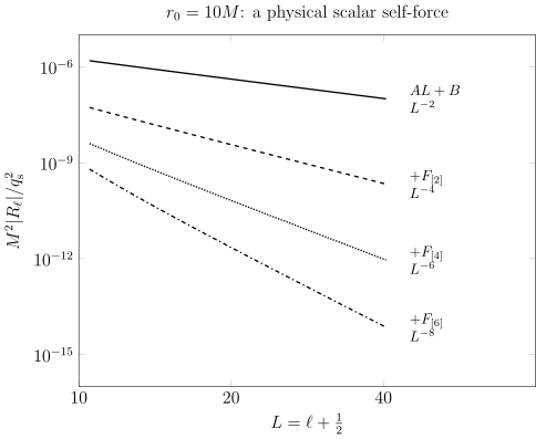
Successive subtraction accelerates the same retarded scalar calculation at $r_0=10M$, with $G=c=1$. Both axes are logarithmic; the vertical axis is the absolute covariant radial-force residual $M^2|R_\ell|/q_{\rm s}^2$ and $L=\ell+1/2$. Curves contain computed multipoles $10\le\ell\le40$. The labels denote cumulative subtraction of the complete, multipole-dependent functions, and the indicated powers are their large-$L$ limits. These are physical mode data with ingoing horizon and outgoing infinity conditions, not a manufactured sequence.

Once modeled with these rational functions, the omitted tail can be summed without numerical integration. For cutoff $N$, define

$$T_k(N)=\frac{N+1}{(2k-1)\displaystyle\prod_{j=1}^k [(2N+2)^2-(2j-1)^2]}.$$

The identity $T_k(N-1)-T_k(N)=b_k(N)$ and the limit $T_k(\infty)=0$ imply $\sum_{\ell\gt N}b_k(\ell)=T_k(N)$ by telescoping. The calculation fits the remaining modes to $b_4,b_5,b_6,b_7$ on $25\le\ell\le40$ and adds the corresponding exact tails.

Results and independent comparisons

The raw modes at 6M, raw modes at 10M, and subtractions and numerical checks retain the inputs needed to repeat the sums. The tail-corrected point estimates are

Radius	$M^2F_r/q_{\rm s}^2$	Empirical convergence allowance
$6M$	$1.67728340233\times10^{-4}$	$2\times10^{-15}$
$10M$	$1.3784482575668\times10^{-5}$	$2\times10^{-18}$

For a quick reanalysis, save those two raw-mode files, the parameters, the checks file, and the analysis script in one folder. With Python and mpmath==1.3.0 installed, run

python analyze_modes.py --compare-directory . --output checks-recomputed.json

This recomputes the subtractions, tail fits and refinement comparisons from the retained inputs. It needs neither Mathematica nor a field solver. The README separately explains how to regenerate the radial solutions. The full-regeneration drivers are the Python radial solver, Mathematica high-precision solver, and parameter exporter.

These allowances exceed the observed precision, cutoff and tail-fit changes described below. They are not total validated error bounds: a method can converge to a biased value, and possible stable or shared solver bias is not bounded here. At $10M$, the result agrees within this allowance with the independent published value $0.000013784482575667959(3)$ in Heffernan, Ottewill, and Wardell 2012, § V F, p. 27. Their parenthesis estimates the finite-mode tail error, not every numerical error. At $6M$ it also reproduces the seven significant figures of the Schwarzschild entry in Warburton and Barack 2010, Table III, p. 15, PDF.

A second comparison holds the cutoff fixed. The thirty-mode calculation in Warburton and Wardell 2014, Table I and following paragraph, p. 10, PDF uses $\ell=0,\ldots,29$. Summing the present order-6 residual only over those same modes gives $0.0001677283080352924$ at $6M$ and $0.00001378448223382866$ at $10M$, reproducing the printed table values. Their difference from the table above is the omitted tail. Agreement between two methods at the same cutoff does not by itself establish the accuracy of the infinite sum.

The external check is weaker at $6M$: that thirty-mode table is rounded at $10^{-14}$ in the force, and the cited full-force result has seven significant figures. Neither independently validates the $2\times10^{-15}$ convergence allowance as a total error estimate.

Convergence checks and their limits

The Python and Mathematica instructions pin the public solver versions and parameter-source revision. A fast double-precision run reaches $\ell=80$; paired higher-precision runs reach $\ell=40$. Increasing the base working precision from 35 to 55 digits tests the cancellation that produces the small residuals. Direct radial-series evaluations are checked against a separate numerical method; discrepant modes are recomputed with the toolkit’s numerical-integration method, and unresolved disagreement stops the calculation.

The following checks probe different numerical failure modes:

• Asymptotic powers. Fits to $20\le\ell\le35$ and $25\le\ell\le40$ recover the predicted $L^{-2}$ and $L^{-4}$ behavior within $0.15$ in exponent. The shifted window checks that a short accidental trend is not mistaken for the asymptotic regime.
• Cutoff and tail fit. The higher-precision cutoff increases from 35 to 40. At fixed cutoff, the tail window and the number of fitted functions are varied independently. All changes are smaller than the convergence allowances above. The 80-mode double-precision run corroborates the trend but cannot establish those smaller allowances as total error estimates.
• Precision and radial sides. Raising working precision by 20 digits preserves the quoted digits. The outer and inner regularized sums agree; their raw difference satisfies the analytically fixed source jump.
• Boundary solutions and flux. The weighted Wronskian is constant to better than $10^{-12}$ relative in the fast calculation. At the same $\ell\le30$ cutoff, a separate point-source flux calculation agrees with $F_t/u^t$ to better than $10^{-12}$ relative at both radii. For this helically symmetric circular scalar field the particle’s rest mass is constant, so positive horizon-plus-infinity energy flux equals $F_t/u^t$, the loss of particle Killing energy per coordinate time.

A deliberately reversed sign of $A_{r,+}$ leaves growing modes, so a failure cannot be hidden by a superficially smooth tail fit. Together these tests support the stated scalar benchmark. Gravitational self-force calculations need their own field equations, completion modes and gauge treatment.

Gauge, basis, and recognizable failures

For the gravitational self-force, the standard Lorenz-gauge prescription assumes a sufficiently regular metric perturbation. The fixed-background scalar calculation above requires no metric-perturbation gauge choice. A radiation-gauge reconstruction may possess a string or a jump through the particle. In a no-string construction the physical prescription generally uses an average of two sides plus an explicitly derived gauge correction; inserting Lorenz-gauge parameters into one radiation-gauge side is unjustified. Likewise, Kerr field solvers naturally use spin-weighted spheroidal harmonics, whereas local parameters are often supplied in spherical harmonics. The coupling transformation must be performed before the $\ell$ limit is interpreted.

Failure signatures are diagnostic. A wrong $A_{\alpha,\pm}$ leaves residual modes growing linearly with $L$; a wrong $B_\alpha$ leaves a nonzero constant; an incorrect $C_\alpha$ leaves a harmonic $1/L$ tail whose partial sums grow logarithmically. A harmonic-normalization error typically rescales both retarded modes and some, but not necessarily all, analytical parameters. Using geodesic-orbit parameters for an accelerated self-consistent orbit changes the local geometry being subtracted. In a gravitational reconstruction, omitting the nonradiative $\ell=0,1$ completion can leave a seemingly well-converged but physically wrong conservative result. Finally, too many fitted tail coefficients can reproduce the final computed modes almost exactly while extrapolating catastrophically; predicted asymptotic powers and fit-window stability are essential.

Mode sum and puncture evolution are complementary. Effective-Source and Puncture Methods solve directly for a residual field, while Gauge-Invariant Self-Force Observables explains which regularized combinations survive admissible gauge changes.

Exercise

Suppose a correctly leading-regularized sequence is

$$R_\ell=\frac{6}{L^2}-\frac{10}{L^4}+O(L^{-6}).$$

Determine the truncation-error scaling before and after subtracting the known $6/L^2$ term. Then suppose the leading parameter was entered as $A+\delta A$. What large-$L$ behavior would reveal the error?

Solution

Since $\sum_{\ell\gt N}L^{-p}=O(N^{1-p})$ for $p\gt 1$, the original tail is

$$\sum_{\ell\gt N}R_\ell=O(N^{-1}).$$

After subtracting $6/L^2$ mode by mode and restoring its exact infinite sum, the remaining sequence begins at $-10/L^4$, so its omitted tail is $O(N^{-3})$. If $A+\delta A$ is subtracted instead of $A$, the residual acquires

$$-\delta A\,L.$$

It therefore grows linearly rather than decaying. Its partial sum grows quadratically with $N$, an unmistakable failure that no inverse-power tail fit can repair.

References

• Barack, Leor, and Amos Ori. “Mode Sum Regularization Approach for the Self Force in Black Hole Spacetime.” Physical Review D 61, 061502(R) (2000). doi:10.1103/PhysRevD.61.061502.
• Barack, Leor, Yasushi Mino, Hiroyuki Nakano, Amos Ori, and Misao Sasaki. “Calculating the Gravitational Self-Force in Schwarzschild Spacetime.” Physical Review Letters 88, 091101 (2002). doi:10.1103/PhysRevLett.88.091101.
• Black Hole Perturbation Toolkit. “Teukolsky,” “pybhpt,” and “RegularizationParameters.” Project documentation and public software, accessed September 19, 2026. Teukolsky; pybhpt; regularization parameters. Exact revisions are recorded in the downloadable calculation.
• Heffernan, Anna, Adrian Ottewill, and Barry Wardell. “High-Order Expansions of the Detweiler–Whiting Singular Field in Schwarzschild Spacetime.” Physical Review D 86, 104023 (2012). doi:10.1103/PhysRevD.86.104023. Open PDF, arXiv v4.
• Warburton, Niels, and Barry Wardell. “Applying the Effective-Source Approach to Frequency-Domain Self-Force Calculations.” Physical Review D 89, 044046 (2014). doi:10.1103/PhysRevD.89.044046. Open PDF, arXiv v3.
• Warburton, Niels, and Leor Barack. “Self Force on a Scalar Charge in Kerr Spacetime: Circular Equatorial Orbits.” Physical Review D 81, 084039 (2010). doi:10.1103/PhysRevD.81.084039. Open PDF, arXiv v3.