Zoom–Whirl Dynamics Near Separatrices

A near-critical encounter approaches an unstable circular or spherical orbit, remains near it for many revolutions, and eventually escapes or plunges. The number of “whirls” grows logarithmically as the invariant impact parameter or angular momentum approaches its critical value. The coefficient is set by the ratio of the orbit’s azimuthal frequency to its radial Lyapunov exponent.

Helpful background. The Einstein Equation fixes the spacetime, Weak Metric Perturbations and Gauge Freedom supplies perturbative comparisons, Presymplectic Potentials and Currents supplies invariant charges, Computational Relativity supplies nonlinear benchmarks, Relativistic Two-Body Dynamics supplies scattering variables, and Black-Hole Geometry and Mechanics supplies unstable orbits.

Expansion about an unstable orbit

Let a conservative radial equation in asymptotic time be

$$\dot r^2=\mathcal R(r;E,J).$$

At the critical orbit,

$$\mathcal R(r_c;E,J_c)=0, \qquad \partial_r\mathcal R(r_c;E,J_c)=0.$$

Write $x=r-r_c$ and $\delta J=J-J_c$. To leading order,

$$\dot x^2 \simeq \lambda_t^2x^2+C\,\delta J,$$

where $\lambda_t\gt 0$ is the radial instability exponent measured in the same asymptotic time as the azimuthal frequency $\Omega_{\phi,c}$. At exact criticality,

$$x(t)\propto e^{\pm\lambda_t t}.$$

A near-critical trajectory enters with radial displacement of order $\sqrt{\lvert\delta J\rvert}$ and leaves when $x$ becomes order unity in the local scaling. Evolution from the minimum displacement to a fixed matching radius contributes $-(2\lambda_t)^{-1}\ln\lvert\delta J\rvert$ on each local leg. The incoming and outgoing legs of a scattering orbit—or the two sides of the near-critical bottleneck for a transmitted orbit—therefore give the full residence time

$$T_{\mathrm{whirl}} \simeq -\frac{1}{\lambda_t} \ln\left\lvert \frac{J-J_c}{J_0} \right\rvert +O(1),$$

where $J_0$ depends on how the local and outer trajectories are matched.

Logarithmic whirl count and scattering angle

During the near-circular segment, $\dot\phi\simeq\Omega_{\phi,c}$. The whirl count is

$$N_{\mathrm{whirl}} =\frac{\Delta\phi_{\mathrm{whirl}}}{2\pi} \simeq -\frac{\Omega_{\phi,c}}{2\pi\lambda_t} \ln\left\lvert \frac{J-J_c}{J_0} \right\rvert +O(1).$$

Consequently the conservative scattering angle has a logarithmic divergence,

$$\chi(E,J) \simeq -\frac{\Omega_{\phi,c}}{\lambda_t} \ln\left\lvert \frac{J-J_c}{J_0} \right\rvert +\chi_0(E).$$

The additive constants depend on the outer orbit and convention used to subtract a straight path. The logarithmic slope is controlled by invariant frequencies normalized to the same asymptotic clock.

The frequency-to-instability ratio is derived explicitly for equatorial Kerr geodesics in Pretorius and Khurana 2007, § IV.A, Eqs. (16)–(19), Open PDF pp. 6–7. Bound zoom–whirl orbits also underlie the periodic-orbit taxonomy of Levin and Perez-Giz 2008, §§ II–IV.

A quantitative Schwarzschild example

Take a massive test particle with specific energy $\mathcal E=3/\sqrt7$ and dimensionless angular momentum $j=\ell/(GM)$. The double-root criterion gives $r_c=7GM/2$ and $j_c=7/\sqrt2$. In terms of $\rho=r/(GM)$, the proper-time radial potential is

$$V(\rho)=\left(1-\frac2\rho\right) \left(1+\frac{j^2}{\rho^2}\right).$$

Differentiating twice at the critical orbit and converting proper time to asymptotic time using $dt/d\tau=\mathcal E/(1-2/\rho_c)$ gives

$$\Omega_{\phi,c}=\frac{1}{GM\rho_c^{3/2}}, \qquad \lambda_t=\Omega_{\phi,c}\sqrt{\frac6{\rho_c}-1}.$$

Both quantities have dimensions of inverse time; their ratio here is $\sqrt{7/5}$. Thus the coefficient of $-\ln\delta$, for $\delta=j/j_c-1\gt0$, is $\sqrt{7/5}/(2\pi)\simeq0.188315$ in the winding count. For a logarithm to base ten, multiply this slope by $\ln10$.

To compute the complete orbit rather than just its near-critical segment, put $u=GM/r$. Eliminating proper time yields

$$\left(\frac{du}{d\phi}\right)^2=P(u), \qquad P(u)=2u^3-u^2+\frac{2u}{j^2}+\frac{\mathcal E^2-1}{j^2}.$$

If $u_p$ is the first positive root reached from $u=0$, then $\Delta\phi=2\int_0^{u_p}du/\sqrt{P(u)}$. The square-root endpoint can be removed by $u=u_p(1-s^2)$ before quadrature. This is also a useful numerical lesson: resolving a turning point analytically is more reliable than asking a uniform radial grid to approximate a singular integrand.

The figure shows one of these orbits and the growth of the total winding $N_{\mathrm{total}}=\Delta\phi/(2\pi)$. Its additive outer-orbit contribution differs from a locally defined whirl count, but its limiting logarithmic slope is the same. Several near-circular revolutions almost overlap in a spatial plot, so the unwrapped angle in the lower panel is the more useful measure.

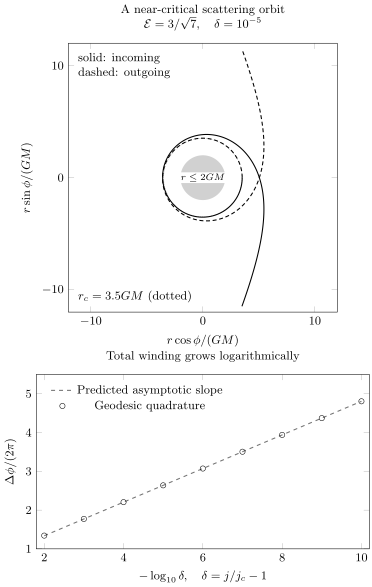
At fixed $\mathcal E=3/\sqrt7$, decreasing $\delta=j/j_c-1$ produces logarithmic growth of the total azimuthal advance. The upper panel shows the $\delta=10^{-5}$ orbit only for $r\leq12GM$ in Schwarzschild polar coordinates; it is not a spatial embedding. The lower points include the complete incoming and outgoing legs to infinity. The dashed guide has slope $\sqrt{7/5}\ln10/(2\pi)$ and is anchored to the last point. These are quantitative test-particle results without radiation reaction.

$\delta$	Periapsis $r_p/(GM)$	$N_{\mathrm{total}}$
$10^{-2}$	3.930809	1.341606
$10^{-4}$	3.538791	2.204913
$10^{-6}$	3.503839	3.072074
$10^{-8}$	3.500383	3.939295
$10^{-10}$	3.500038	4.806516

The downloadable Python calculation runs with Python 3 and mpmath==1.3.0. It compares 40- and 65-digit quadratures, an elliptic-integral evaluation, and a separate Runge–Kutta integration of $u''=-u+j^{-2}+3u^2$ at three step sizes for the first three tabulated offsets ($10^{-2},10^{-4},10^{-6}$). The last two tabulated points give slope $0.188314666$ against $-\ln\delta$, approaching the predicted $0.188314668$. These checks concern the stated geodesic problem; they do not bound the error of an EOB or comparable-mass model.

What should be measured

To test the scaling, hold invariant incoming energy fixed and vary invariant $J$ or $b=J/p_\infty$. For each scattering trajectory:

1. extract the total unwrapped azimuthal advance or scattering angle;
2. fit it against $\ln\lvert J-J_c\rvert$;
3. determine $\Omega_{\phi,c}$ and $\lambda_t$ independently from the critical orbit;
4. compare the fitted and predicted slopes;
5. vary the fit window and exclude points whose uncertainty in $J-J_c$ dominates the abscissa.

Counting coordinate loops by eye is less robust. A gauge transformation can distort the plotted path while leaving the asymptotic angle and critical frequency ratio unchanged.

In numerical relativity, finite extraction radius, junk radiation, and uncertainty in incoming invariants become strongly amplified near threshold. Both axes have correlated errors, so ordinary least squares is generally inadequate. A fit should propagate the covariance and report whether the critical value was calibrated on or independently predicted for the sequence.

Radiation and finite-size limits

The conservative logarithm cannot grow indefinitely in a physical dissipative encounter. Each whirl radiates energy and angular momentum, changing both the orbit and the conservative separatrix appropriate to its instantaneous energy. Define the signed distance $D=J-J_c(E)$. If energy and angular-momentum losses per orbit are $\Delta E_{\mathrm{rad,orbit}}$ and $\Delta J_{\mathrm{rad,orbit}}$, a local small-drift condition is

$$N_{\mathrm{whirl}}\, \left\lvert\Delta J_{\mathrm{rad,orbit}} -J_c'(E)\Delta E_{\mathrm{rad,orbit}}\right\rvert \ll\lvert J-J_c\rvert.$$

This assumes the loss rates and $J_c'$ change little over the segment. On a circular family, $dE=\Omega_c\,dJ_c$, so $J_c'=1/\Omega_c$. Nearly circular radiation satisfying $\Delta E\simeq\Omega_c\Delta J$ can cancel the leading drift in $D$; the size of $\Delta J$ alone therefore does not determine when the orbit crosses the separatrix. Once the coupled energy–angular-momentum evolution changes the local orbit substantially, it must be evolved through the whirl rather than applied afterward. Tidal excitation, horizon absorption, and spin precession can be enhanced by the same residence time. Near-critical sensitivity therefore narrows the useful domain of every finite-order point-particle approximation.

The logarithmic law remains a local organizing principle, but its critical parameters and cutoff change in a comparable-mass, spinning, or dissipative system. Finite-amplitude merger dynamics is not predicted by the geodesic formula.

A useful final check approaches criticality from both sides. The scatter side and plunge side should yield the same local logarithmic slope while differing in their outer additive constants and final outcomes. A slope that changes under modest window refinement usually signals dissipation, unresolved critical data, or departure from the asymptotic region.

Exercises

Derive the logarithmic residence time from exponential radial departure.

Solution

If the entry displacement scales as $x_{\mathrm{in}}\propto\sqrt{\lvert J-J_c\rvert}$ and $x=x_{\mathrm{in}}e^{\lambda_t t}$, reaching fixed $x_{\mathrm{out}}$ on one leg takes

$$t =\frac{1}{\lambda_t} \ln\frac{x_{\mathrm{out}}}{x_{\mathrm{in}}} =-\frac{1}{2\lambda_t} \ln\lvert J-J_c\rvert+O(1).$$

The near-critical portion of a complete scattering orbit has an incoming and an outgoing leg. Adding them gives

$$T_{\mathrm{whirl}} =-\frac{1}{\lambda_t}\ln\lvert J-J_c\rvert+O(1),$$

in agreement with the main result. The factor of two counts orbit segments; it is not a redefinition of the physically fixed exponent in $x\propto e^{\pm\lambda_t t}$. A different control parameter can change the reported slope only through an explicitly stated nonlinear map to $J-J_c$.

Why must $\Omega_{\phi,c}$ and $\lambda_t$ use the same time parameter?

Solution

Under a constant rescaling of time, each frequency rescales inversely, so their ratio is unchanged. Mixing a proper-time Lyapunov exponent with an asymptotic-time azimuthal frequency lacks that cancellation and gives a spurious slope.

References

• Levin, Janna, and Gabe Perez-Giz. “A Periodic Table for Black Hole Orbits.” Physical Review D 77 (2008): 103005. DOI.
• Pretorius, Frans, and Deepak Khurana. “Black Hole Mergers and Unstable Circular Orbits.” Classical and Quantum Gravity 24 (2007): S83–S108. DOI. Open PDF, arXiv v2.