Branch-Cut Contributions to Retarded Response

A branch cut contributes a continuous range of frequencies to a retarded response. Its endpoint can therefore produce a power-law tail after damped resonances have faded—but the power, coefficient, and even the presence of that tail depend on the discontinuity, initial data, and observation limit. This page derives the endpoint rule, distinguishes logarithms in a resolvent from logarithms in its jump, and checks the orientation and causal support in an exactly solvable one-dimensional massive wave problem.

Required background. PDEs and Green Functions for Gravitation supplies causal Green functions, Laplace inversion, and Wronskians.

Helpful background. Black-Hole Geometry and Mechanics supplies the horizon and asymptotic ends; Formulations of General Relativity supplies field-specific master equations; Causality and Global Structure distinguishes retarded support and observation regions; Black-Hole Perturbation Theory supplies the surrounding spectral decomposition.

The radial resolvent and genuine singularities

Write a real, time-independent separated wave operator as $P=\partial_t^2+A$, where $A=-\partial_x^2+V(x)$ and $x=r_*$ in the black-hole application. Use the positive-wave source normalization of Price-Law Tails in Schwarzschild:

$$PG(t;x,x')=\delta(t)\delta(x-x'), \qquad G=0\quad(t\lt0).$$

The Laplace variable $s=-i\omega$ has dimensions of inverse length. In a right half-plane where the transform exists, its kernel $H$ obeys

$$(A+s^2)H(s;x,x')=\delta(x-x').$$

Let $u_L$ and $u_R$ satisfy the retarded left and right boundary conditions, initially fixed by decay at their respective ends in that half-plane. For a massless asymptotically flat problem these continue the horizon-ingoing and infinity-outgoing solutions. Put $x_< =\min(x,x')$ and $x_> =\max(x,x')$. Their constant Wronskian and kernel are

$$\begin{aligned} W(s)&=u_Lu_R'-u_Ru_L',\\ H(s;x,x')&=-\frac{u_L(s,x_<)u_R(s,x_>)}{W(s)},\\ \partial_xH\big|_{x=x'+0}-\partial_xH\big|_{x=x'-0}&=-1. \end{aligned}$$

The last line follows by integrating $-\partial_x^2H=\delta+\text{regular}$ across the source; it fixes the overall sign. The detailed construction is developed in Mode Green Functions and Wronskians. Casals and Ottewill write the negative-wave operator with a negative delta source: reversing both sides yields this same kernel, without a kernel sign change. See Casals and Ottewill 2015, § II A, p. 3, Eqs. (2.6)–(2.8), Open PDF.

Away from thresholds, a simple zero of $W$ gives a simple pole of the complete kernel when the two endpoint solutions are nonzero and holomorphic there and the numerator does not cancel it. Multiplying an endpoint solution by a vanishing normalization can instead create a removable Wronskian zero. A threshold or a higher-order zero needs a separate local expansion. Even a genuine operator pole can disappear from a particular measured response when its source or observation projection vanishes. Thus a denominator zero alone is not a resonance test.

For smooth compact initial displacement $h(x)$ and velocity $g(x)$, the homogeneous solution is

$$\psi(t,x)=\int_{\mathbb R} \left[G(t;x,x')g(x')+\partial_tG(t;x,x')h(x')\right]dx'.$$

Equivalently, its transformed source is $g+s h$. When discussing a chosen field value or other linear observation after this convolution, write $X(t)$ and $\widehat X(s)$; neither is the two-point kernel $G$.

Deforming the retarded contour

Take $\gamma$ to the right of the response’s growth bound, not merely to the right of zero if unstable modes are possible. The upward Bromwich integral is

$$X(t)=\frac{1}{2\pi i} \int_{\gamma-i\infty}^{\gamma+i\infty} e^{st}\widehat X(s)\,ds.$$

First deform a finite contour. Keep the crossed residues, both banks of every cut, and the remaining arcs; only then take limits justified by estimates. For a cut on the negative real $s$ axis define

$$\Delta\widehat X(-\sigma) =\widehat X(-\sigma-i0)-\widehat X(-\sigma+i0), \qquad \sigma\gt0.$$

The small clockwise boundary surrounding the excluded cut runs toward the endpoint on its upper bank and away on its lower bank. Subtracting that boundary from the enclosing contour gives

$$X_{\mathrm{cut}}(t) =\frac{1}{2\pi i}\int_0^\infty e^{-\sigma t}\Delta\widehat X(-\sigma)\,d\sigma.$$

This sign also follows from the following rotation of the frequency plane.

Frequency-plane bank at the downward cut	Image under $s=-i\omega$
East: $\omega=+\epsilon-i\sigma$	Lower: $s=-\sigma-i\epsilon$
West: $\omega=-\epsilon-i\sigma$	Upper: $s=-\sigma+i\epsilon$

Thus east minus west in the frequency plane is lower minus upper in the Laplace plane. The same cut normalization appears in Casals and Ottewill 2015, § II A, p. 5, Eqs. (2.19)–(2.21), Open PDF. Leaver’s upper-minus-lower integral runs from $0$ to $-\infty$; changing to positive $\sigma$ gives the sign above. His decomposition explicitly retains a high-frequency part alongside poles and the cut: Leaver 1986, § II B, author-version p. 7, Eqs. (22)–(24), Open PDF.

In the following frequency-plane diagram, inspect the arrows on the two banks and the retained large-frequency segment. The diagram shows the conventional Schwarzschild cut, not the finite massive cut calculated below.

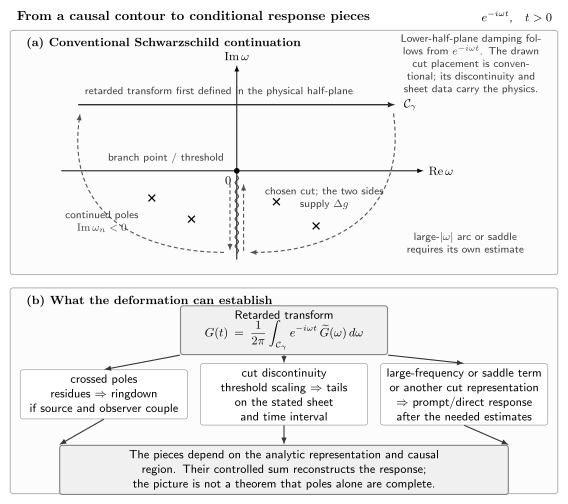
Schematic retarded contour for $e^{-i\omega t}$ and $t\gt0$, not to scale. On the conventional Schwarzschild sheet shown here, lowering the physical upper-half-plane line crosses specified damped poles and follows both banks of a negative-imaginary-axis cut. Residues can generate ringdown, threshold discontinuities can generate tails, and the prompt/direct part may be carried by a large-frequency contribution or by a different cut representation. This is not a pole-completeness statement: each arc, sheet, orientation, and causal-region assumption still requires proof.

The large-frequency contribution need not vanish just because $t\gt0$. Propagation distances also enter the exponential factors. Neither the picture nor an endpoint expansion proves that a pole-plus-cut expression converges for arbitrary data or at arbitrary times.

Endpoint powers and a controlled remainder

Define the normalized, data-projected density $\rho(\sigma)=\Delta\widehat X(-\sigma)/(2\pi i)$. Here is a sufficient hypothesis for a precise endpoint estimate. For some fixed $\sigma_0\gt0$, assume

$$\rho(\sigma)=a\sigma^p+R(\sigma), \qquad |R(\sigma)|\le C\sigma^{p+\eta}, \qquad 0\lt\sigma\lt\sigma_0, \quad p\gt-1,\quad\eta\gt0,$$

and, for some fixed $t_b\gt0$, assume

$$B=\int_{\sigma_0}^{\infty} e^{-t_b\sigma}|\rho(\sigma)|\,d\sigma\lt\infty.$$

Split the cut integral at $\sigma_0$. The far piece is bounded by $B e^{-(t-t_b)\sigma_0}$ for $t\ge t_b$. The local remainder is bounded by $C\Gamma(p+\eta+1)t^{-p-\eta-1}$, and extending the leading monomial from $\sigma_0$ to infinity makes only an exponentially small error. With $z=\sigma t$, the remaining integral is

$$\int_0^\infty e^{-\sigma t}\sigma^p\,d\sigma =\Gamma(p+1)t^{-p-1}.$$

Consequently,

$$X_{\mathrm{cut}}(t) =a\Gamma(p+1)t^{-p-1} +O(t^{-p-\eta-1}).$$

This is an elementary form of Watson’s lemma; compare NIST DLMF 2026, § 2.3(ii), Eq. (2.3.8). If $a=0$, this formula gives a bound, not the next nonzero power. The constants and assumptions refer to the declared observation and source class. Moving the observation point toward null infinity need not preserve them.

The conclusion controls this cut contribution. Other endpoints, unstable or undamped poles, and unestimated arcs may change the full late-time response. A nonzero endpoint term on the imaginary axis outlasts a fixed isolated damped pole, but this comparison alone does not control an infinite pole sum. A cut starting at $s_0$ rather than zero carries the additional factor $e^{s_0t}$ and, for a nonreal $s_0$, an oscillatory phase.

Logarithms in the resolvent and in the jump

Introduce a fixed length $L\gt0$ so that every logarithm has a dimensionless argument. Define the digamma function by $\Psi(z)=\Gamma'(z)/\Gamma(z)$, distinct from the wave field $\psi$. Differentiating the convergent gamma integral with respect to $p$ gives

$$\int_0^\infty e^{-\sigma t}\sigma^p\log(\sigma L)\,d\sigma =\Gamma(p+1)t^{-p-1} \left[\Psi(p+1)-\log(t/L)\right].$$

The same local/far splitting controls a logarithmic endpoint expansion; see NIST DLMF 2026, § 2.3(ii), Eq. (2.3.9). It is a logarithm in the discontinuity that produces the logarithm in time. To see why the distinction matters, take the principal logarithm with the negative-real-axis cut. For an integer $n\ge0$,

$$\begin{aligned} \log[(-\sigma\mp i0)L]&=\log(\sigma L)\mp i\pi,\\ \Delta\!\left[s^n\log(sL)\right] &=-2\pi i(-1)^n\sigma^n,\\ \Delta\!\left[s^n\log^2(sL)\right] &=-4\pi i(-1)^n\sigma^n\log(\sigma L). \end{aligned}$$

A single resolvent logarithm times an integer power therefore produces a pure-power jump; a squared logarithm produces a logarithmic jump. Terms analytic through the cut have no local discontinuity. A polynomial in $s$, considered as a full transform, contributes only contact distributions at $t=0$; an arbitrary locally analytic part is not thereby proved irrelevant to the whole contour. These statements concern local expansions, not permission to replace the full resolvent at every frequency.

For the fixed-radius Schwarzschild scalar modes with $\ell\ge1$, the normalized cut density contains terms proportional to $\sigma^{2\ell+2}$, $\sigma^{2\ell+3}$, and $\sigma^{2\ell+4}\log(2GM\sigma)$. The last gives a $t^{-2\ell-5}\log[t/(2GM)]$ correction, two inverse powers beyond the leading Price tail. The quantities and radial factors must be combined before inversion; the intermediate Bardeen–Press–Teukolsky expansion explicitly excepts the scalar monopole. See Casals and Ottewill 2015, § VII A, pp. 31–32, Eqs. (7.1)–(7.5), Open PDF. Data convolution can subsequently cancel a coefficient; the kernel expansion is not an assertion that every solution has every listed term.

A solvable massive radial problem

An exact example tests more than formal power counting. On the full line, take the free one-dimensional massive operator

$$(\partial_t^2-\partial_x^2+m^2)G(t;x,x') =\delta(t)\delta(x-x'), \qquad m\gt0,\qquad d=|x-x'|.$$

Here $m$ is a mass parameter with dimensions of inverse length, not an angular index. There is no black-hole potential or angular barrier. This is the model in Analytic Structure: Poles, Cuts, and Thresholds, with its negative-wave, positive-source kernel multiplied by $-1$ to obtain the positive-wave, positive-source kernel used here.

The outgoing sheet and its two banks

Choose the branch $\kappa(s)^2=s^2+m^2$ analytic outside the finite vertical segment $i[-m,m]$, with $\kappa(s)\sim s$ at infinity. It has $\operatorname{Re}\kappa\gt0$ in the right half-plane. The decaying endpoint solutions there give

$$u_L=e^{\kappa x}, \qquad u_R=e^{-\kappa x}, \qquad W=-2\kappa, \qquad H(s;d)=\frac{e^{-\kappa d}}{2\kappa}.$$

Continue this same branch around the endpoints. Do not choose a fresh decaying square root on the west bank: that changes the continued problem. For $s=iy$, $-m\lt y\lt m$, put $\chi=\sqrt{m^2-y^2}\gt0$. The bank values are

$$\begin{aligned} \kappa_E&=+\chi, & H_E&=\frac{e^{-\chi d}}{2\chi},\\ \kappa_W&=-\chi, & H_W&=-\frac{e^{+\chi d}}{2\chi},\\ H_E-H_W&=\frac{\cosh(d\chi)}{\chi}. \end{aligned}$$

The finite segment is a choice of chart for the outgoing continuation. It does not assert that propagating real frequencies lie between $-m$ and $m$: their wavenumber is real for $|\omega|\gt m$.

Exact inversion and causal arrival

For $t\gt d$, closing the Bromwich line to the left leaves the east bank upward minus the west bank upward. Since $ds=i\,dy$, the result is

$$G_{\mathrm{cut}}(t;d) =\frac{1}{2\pi}\int_{-m}^{m} e^{iyt}\frac{\cosh\!\left(d\sqrt{m^2-y^2}\right)} {\sqrt{m^2-y^2}}\,dy.$$

Set $y=m\cos\theta$; this removes both endpoint singularities. The integral becomes half a full-circle average of $\exp(imt\cos\theta+md\sin\theta)$. Expanding that entire function and integrating the angular powers, or analytically continuing Bessel’s integral, gives

$$G(t;d)=\frac12\Theta(t-d) J_0\!\left(m\sqrt{t^2-d^2}\right).$$

The expression is defined piecewise: it is zero before arrival and the displayed Bessel function after arrival. Its value exactly at the wavefront does not affect its distributional definition. For the Bessel integral see NIST DLMF 2026, Eq. (10.9.1). One can independently check the source: with $u=t-(x-x')$, $v=t+(x-x')$ and $F(w)=J_0(m\sqrt w)$, the interior equation is $4(wF''+F')+m^2F=0$. Acting on $\Theta(u)\Theta(v)F(uv)/2$ leaves $2\delta(u)\delta(v)=\delta(t)\delta(x-x')$, since $F(0)=1$. This verifies both causality and normalization.

The cut integral alone, however, is nonzero when $0\lt t\lt d$:

$$G_{\mathrm{cut}}(t;d) =\frac12 I_0\!\left(m\sqrt{d^2-t^2}\right), \qquad 0\lt t\lt d.$$

Here $I_0(z)=J_0(iz)$. Before arrival, the large-frequency contribution cannot be discarded; it cancels this cut value. Indeed $e^{st}H\sim e^{s(t-d)}/(2s)$ at large $s$ on this sheet, so the leftward closure decays only after the propagation time $d$. The causal step function is not an optional correction to a tail formula.

Threshold power and phase

Keep $m\gt0$ and $d$ fixed and let $t\to\infty$. Near the upper endpoint write $y=m-\eta$. Then

$$\frac{\cosh(d\chi)}{\chi} =(2m\eta)^{-1/2}\,[1+O(\eta)].$$

With a smooth endpoint cutoff, the leading oscillatory integral is evaluated by adding a positive convergence factor and then removing it:

$$\lim_{\epsilon\downarrow0} \int_0^\infty e^{-(\epsilon+it)\eta}\eta^{-1/2}\,d\eta =\sqrt{\pi}\,e^{-i\pi/4}t^{-1/2}.$$

It supplies $e^{i(mt-\pi/4)}/[2\sqrt{2\pi mt}]$. The lower endpoint supplies its complex conjugate. Smooth interior terms can be integrated by parts, and the next endpoint powers are $\eta^{1/2}$. Thus

$$G(t;d)=\frac{\cos(mt-\pi/4)}{\sqrt{2\pi mt}} +O(t^{-3/2}), \qquad m\gt0,\quad d\ \text{fixed}.$$

This agrees independently with the large-argument expansion of the exact Bessel result: NIST DLMF 2026, Eq. (10.17.3). The error is absolute, not relative to a cosine that vanishes repeatedly. The constant in the error depends on the fixed parameters. Neither a limit along the wavefront nor $m\to0$ is covered by this expansion. In fact the exact massless limit is $\Theta(t-d)/2$, so the zero-mass and late-time limits cannot be interchanged.

The $t^{-1/2}$ envelope belongs to this free one-dimensional threshold. It is not the curvature-induced $t^{-5/6}$ asymptotic law discussed in Massive Fields and Oscillatory Tails.

Checking a cut calculation

A useful numerical test follows the same continued branch to matched points on both banks, decreases the distance from the cut, and compares the signed complex difference with the predicted jump. Agreement of magnitudes cannot detect a reversed orientation. For the massive example, the substitution $y=m\cos\theta$ gives a nonsingular quadrature that can be compared with the Bessel result. A separate forward Laplace transform of the causal Bessel kernel must recover $e^{-d\kappa}/(2\kappa)$.

These tests independently check radial normalization, inversion, causal arrival, and endpoint phase; they do not constitute a black-hole evolution. For a black-hole application one must additionally control the radial solutions, data projection, relevant frequency range, and observation limit. A logarithmic-slope fit near zeros of an oscillatory signal is unreliable; fit its phase and envelope or compare absolute errors instead.

Exercises

1. A removable Wronskian zero. For $V=0$ on the full line, start with $u_L=e^{sx}$ and $u_R=e^{-sx}$. Replace $u_L$ by $a(s)u_L$, where $a(s)=L(s-s_0)$ and $s_0\gt0$. Does the new Wronskian predict an instability?

Solution

The original Wronskian is $-2s$. The replacement gives $W_a=-2s\,a(s)$, but also multiplies the numerator by $a(s)$. Away from its zero, and by analytic extension through $s_0$,

$$H_a(s;d)=\frac{a(s)e^{-sd}}{2s\,a(s)} =\frac{e^{-sd}}{2s}.$$

This kernel is regular at $s_0\gt0$, so the new zero is not an unstable pole. The endpoint solution’s normalization vanishes there, violating the nonzero-normalization condition. The distinct zero-frequency singularity at $s=0$ has not been removed.

2. Which logarithm survives inversion? Suppose a local resolvent term is $B s^2\log^2(sL)$, with constant coefficient $B$. Compute its oriented jump and its late-time cut contribution for $t\gt0$, assuming the remainder and other contour pieces are separately controlled. Compare with $B s^2\log(sL)$.

Solution

The normalized jump of the squared-logarithm term is $-2B\sigma^2\log(\sigma L)$. Since $\Gamma(3)=2$,

$$X_{\mathrm{cut}}(t)\ \supset\ -4B\,t^{-3}\left[\Psi(3)-\log(t/L)\right].$$

The single-logarithm term instead has normalized jump $-B\sigma^2$ and contributes $-2Bt^{-3}$, with no time logarithm. These are the contributions of the stated local terms, not a remainder theorem for an unspecified full resolvent.

3. Does initial displacement always gain an inverse power of time? Use real, smooth compact data $h,g$ for the massive full-line model and a fixed observer. Put $M_h=\int h(x')\,dx'$ and $M_g=\int g(x')\,dx'$. Find the leading field, and compare with the zero-frequency endpoint in the preceding Price-law page.

Solution

The Bessel asymptotic expansion is uniform on the compact source support and can be differentiated with its corresponding remainder estimate. Differentiating the leading carrier changes its phase and supplies $m$; it does not supply only $1/t$. The Cauchy formula therefore gives

$$\psi(t,x)= \frac{M_g\cos(mt-\pi/4)-mM_h\sin(mt-\pi/4)} {\sqrt{2\pi mt}} +O(t^{-3/2}).$$

For real data the leading oscillation vanishes identically only when both $M_g=0$ and $M_h=0$. Setting the initial velocity to zero alone leaves a leading $t^{-1/2}$ oscillation if $M_h\ne0$. At a zero-frequency power-law endpoint, in contrast, differentiation of $t^{-p}$ gives $-pt^{-p-1}$, provided the differentiated remainder is controlled. The carrier frequency is the decisive difference. A vanished leading moment still does not identify the next nonzero coefficient.

References

• Casals, Marc, and Adrian C. Ottewill. “High-order Tail in Schwarzschild Space-time.” Physical Review D 92 (2015): 124055. DOI. Open PDF, arXiv:1509.04702v2.
• Leaver, Edward W. “Spectral Decomposition of the Perturbation Response of the Schwarzschild Geometry.” Physical Review D 34 (1986): 384–408. DOI. Open PDF, author version with its own pagination.
• NIST (National Institute of Standards and Technology). Digital Library of Mathematical Functions. §§ 2.3, 10.9, and 10.17. DLMF. Consulted 2026-09-05.