Mode Green Functions and Wronskians

A radial Green function is assembled from two homogeneous solutions, each satisfying one endpoint condition. The value matches continuously at the source, while its derivative jumps by exactly the amount needed to create a delta function. This page derives that normalization for a separated black-hole master equation, then treats weighted radial operators and delta-prime sources. The central lesson is that the operator, source measure, and endpoint normalization form one calculation.

Required background. PDEs and Green Functions for Gravitation supplies distributional matching, Fourier–Laplace transforms, and Green identities.

Helpful background. Black-Hole Geometry and Mechanics fixes the horizon and outer endpoint; Formulations of General Relativity supplies wave operators; Events, Intervals, and Minkowski Geometry fixes causal orientation; Black-Hole Perturbation Theory introduces the master fields.

Radial inverses and endpoint solutions

Start with a massless Schwarzschild master equation in tortoise coordinate $x=r_*$, suppressing the fixed angular labels:

$$[-\partial_t^2+\partial_x^2-V_\ell(x)]\Psi(t,x)=S(t,x).$$

Here $V_\ell$ is a smooth real potential, with the usual decaying Schwarzschild endpoint behavior. Take a smooth compactly supported source that vanishes for $t\leq0$, and zero past field and velocity. This avoids initial-slice source terms and noncompact-source convergence issues; those are separate from the radial matching problem.

For a response growing no faster than $e^{\gamma t}$ in the relevant norm, choose $\eta\gt\max(\gamma,0)$ and use

$$\begin{aligned} \widetilde\Psi(\omega,x) &=\int_0^\infty e^{i\omega t}\Psi(t,x)\,dt,\\ \Psi(t,x) &=\frac1{2\pi}\int_{-\infty+i\eta}^{+\infty+i\eta} e^{-i\omega t}\widetilde\Psi(\omega,x)\,d\omega. \end{aligned}$$

Transform $S$ the same way. The inverse contour runs left to right. Integration by parts has no initial-data term under the stated assumptions, so

$$L_\omega\widetilde\Psi=\widetilde S, \qquad L_\omega=\frac{d^2}{dx^2}+\omega^2-V_\ell(x).$$

We seek $g(x,x';\omega)$ with $L_\omega g=\delta(x-x')$, where the operator acts in $x$ and the source measure is $dx'$. Its inverse transform is the retarded radial kernel. A real-axis $\omega+i0$ prescription is a boundary value of this construction when that limit exists, not a replacement for specifying a convergent initial contour. The preceding retarded Green-function page explains the spacetime existence and boundary assumptions.

Let $u_L$ and $u_R$ solve $L_\omega u=0$, with unit endpoint amplitudes:

$$\begin{aligned} u_L(x,\omega)&\sim e^{-i\omega x} &&(x\to-\infty),\\ u_R(x,\omega)&\sim e^{+i\omega x} &&(x\to+\infty). \end{aligned}$$

In the upper half-plane each selected wave decays at its own endpoint. The horizon wave combines with time as $e^{-i\omega(t+x)}$, regular along ingoing characteristics; the outer wave depends on $t-x$ and is outgoing. Continue these solutions from their initial analytic domain when discussing complex resonances. These pure phases apply to the stated massless Schwarzschild master variable, away from the zero-frequency threshold. Kerr requires the horizon frequency $\omega-m\Omega_H$ and the appropriate spin-dependent radial powers; massive fields require their actual outer wave number and threshold behavior.

Continuity and the unit source jump

For homogeneous solutions define the oriented, unconjugated Wronskian

$$W[u_L,u_R]=u_Lu_R'-u_Ru_L', \qquad W'=u_Lu_R''-u_Ru_L''=0.$$

Primes here denote $x$ derivatives. Both second derivatives equal $(V_\ell-\omega^2)$ times the corresponding solution, so they cancel. This is an algebraic identity between two solutions, not an energy-flux identity involving complex conjugation.

For $W(\omega)\ne0$, impose the left condition below the source and the right condition above it:

$$g(x,x';\omega)= \begin{cases} u_L(x)u_R(x')/W,&x\lt x',\\ u_L(x')u_R(x)/W,&x\gt x'. \end{cases}$$

The two limits agree. Their first derivatives obey

$$[g]_{x'}=0, \qquad [\partial_xg]_{x'} =\frac{u_L(x')u_R'(x')-u_R(x')u_L'(x')}{W}=1,$$

where $[h]_{x'}=h(x'+)-h(x'-)$. A continuous piecewise smooth function has a delta in its second distributional derivative precisely when its first derivative jumps. Thus the homogeneous equation away from $x'$ and this unit jump prove $L_\omega g=\delta$. Equivalently,

$$g(x,x';\omega) =\frac{u_L(x_<,\omega)u_R(x_>,\omega)}{W(\omega)}, \qquad x_<=\min(x,x'),\quad x_>=\max(x,x').$$

The product formula also gives $g(x,x';\omega)=g(x',x;\omega)$ for this scalar problem. This spatial transpose symmetry is not a claim that a retarded spacetime kernel is unchanged when source and observation events are interchanged.

Leaver gives the endpoint construction in Leaver 1986, author PDF, § II A, pp. 5–6, Eqs. (6)–(15). His source is $-\delta$ and his Wronskian order is reversed. With $L=2GM$, his dimensionless coordinate $\bar x=x/L$, and Laplace variable $s=-iL\omega$, the conversion is $W=-W_{\rm Leaver}/L$ and $g=-L g_{\rm Leaver}$. The page numbers in that citation are the author version’s printed labels, not the journal pagination.

An exact free kernel

Set $V_\ell=0$ on the whole line. The endpoint solutions are exact exponentials, and

$$W_0=2i\omega, \qquad g_0(x,x';\omega)=\frac{e^{i\omega|x-x'|}}{2i\omega}.$$

The kernel has units of length: a second derivative then has the same units as the one-dimensional delta. At $\omega=i\kappa$, $\kappa\gt0$, put

$$X=\kappa(x-x'),\qquad Y=\kappa g_0=-\frac12e^{-|X|}.$$

Inspect the common value and the two one-sided tangents in the figure. Since $dY/dX=\partial_xg_0$, their difference is exactly the physical derivative jump.

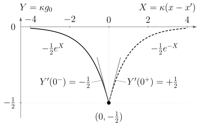
The exact whole-line free kernel at $\omega=i\kappa$, $\kappa\gt0$, is $Y=-e^{-|X|}/2$ with the scaled axes defined above. Its value is continuous at $-1/2$, while the derivative rises from $-1/2$ to $+1/2$, producing the unit delta source. This is a frequency-domain kernel, not a growing time-domain mode or a quasinormal mode.

Source trace	Left limit	Right limit	Right minus left
$Y$	$-1/2$	$-1/2$	$0$
$dY/dX$	$-1/2$	$+1/2$	$1$

For an independent time-domain check, let $\tau=t-t'$ and $d=|x-x'|$. The causal free kernel is $G_0=-\Theta(\tau-d)/2$; directly integrating $-\frac12\int_d^\infty e^{i\omega\tau}\,d\tau$ gives $g_0$ above. Changing the radial operator to $-L_\omega$ while retaining a positive delta changes the Green function to $-g$.

Compact forcing and delta-prime sources

For an ordinary compact radial source, the solution is

$$\begin{aligned} \widetilde\Psi(x) ={}&\frac{u_R(x)}{W} \int_{-\infty}^{x}u_L(x')\widetilde S(x')\,dx'\\ &+\frac{u_L(x)}{W} \int_x^\infty u_R(x')\widetilde S(x')\,dx'. \end{aligned}$$

On differentiating once, the two terms from the moving integration limit cancel. Differentiating again leaves $(u_Lu_R'-u_Ru_L')\widetilde S/W=\widetilde S$ in addition to the homogeneous terms. Beyond the source on the right only $u_R$ remains; beyond it on the left only $u_L$ remains. This both checks the source and explains how its radiation reaches the two endpoints. A source extending to an endpoint needs its own convergence or regularization argument.

Now allow an interior distributional source

$$\widetilde S(x)=A(x)\delta(x-x_p)+F(x)\delta'(x-x_p),$$

with smooth $A,F$ and the prime on the delta denoting its coordinate derivative. The product rule for distributions gives

$$F(x)\delta'(x-x_p)=F(x_p)\delta'(x-x_p)-F'(x_p)\delta(x-x_p).$$

For a piecewise smooth field, writing $J_0=[\widetilde\Psi]_{x_p}$ and $J_1=[\widetilde\Psi']_{x_p}$, the singular part of $L_\omega\widetilde\Psi$ is $J_0\delta'+J_1\delta$. Hence

$$[\widetilde\Psi]_{x_p}=F(x_p), \qquad [\widetilde\Psi']_{x_p}=A(x_p)-F'(x_p).$$

The kernel gives the same field away from the source:

$$\widetilde\Psi(x) =A(x_p)g(x,x_p) -\left.\partial_{x'}[g(x,x')F(x')]\right|_{x'=x_p}, \qquad x\ne x_p.$$

At $x=x_p$, the source-slot derivative has unequal one-sided limits. Use the limiting fields and the jump conditions; the distributional equation does not select a canonical point value there. In particular, dropping $F'(x_p)$ or differentiating only one arbitrary branch of the coincident kernel changes the source.

Weighted radial operators and source measures

The same matching method works before a radial equation has been reduced to Schrödinger form. In a coordinate $q$, let

$$\mathcal D=a_2(q)\frac{d^2}{dq^2} +a_1(q)\frac{d}{dq}+a_0(q), \qquad a_2(q)\ne0,$$

with smooth coefficients on the open interval of interest. Fix one homogeneous condition at each endpoint, assume their solutions $v_L,v_R$ are independent, and define $W_q=v_Lv_R'-v_Rv_L'$. Primes in this section are $q$ derivatives. Substitution gives Abel’s identity:

$$W_q'=-\frac{a_1}{a_2}W_q, \qquad p(q)=\exp\!\int^q\frac{a_1}{a_2}\,d\bar q, \qquad C=pW_q=\text{constant}.$$

If a kernel is integrated against a specified smooth nonzero density $\rho(q')\,dq'$, its defining delta must be normalized accordingly:

$$\begin{aligned} \mathcal D_q g_\rho(q,q')&=\frac{\delta(q-q')}{\rho(q')},\\ g_\rho(q,q') &=\frac{v_L(q_<)v_R(q_>)}{a_2(q')W_q(q')\rho(q')},\\ y(q)&=\int g_\rho(q,q')S(q')\rho(q')\,dq'. \end{aligned}$$

The kernel is continuous and its derivative jumps by $1/[a_2(q')\rho(q')]$, proving the formula directly. In particular, the ordinary coordinate measure has $\rho=1$.

A useful choice is $w=p/a_2$, because

$$\mathcal D y =\frac1w\bigl[(p y')'+w a_0y\bigr], \qquad g_w(q,q')=\frac{v_L(q_<)v_R(q_>)}{C}.$$

This is divergence form, not automatically a self-adjoint operator. The product gives the bilinear symmetry $g_w(q,q')=g_w(q',q)$ for these separated scalar boundary conditions; for the coordinate-measure kernel, $g_1(q,q')/w(q')=g_1(q',q)/w(q)$. A positive Hilbert-space weight, appropriate real coefficients and an adjoint-compatible operator domain require additional analysis. In particular, a complex-frequency pencil or a Teukolsky operator cannot be declared self-adjoint merely because $C$ is constant.

The Teukolsky source weight

For the radial Teukolsky equation, write its already-defined algebraic radial term as $Q_s$:

$$\mathcal D_sR =\Delta^{-s}\frac{d}{dr}\left(\Delta^{s+1}R'\right)+Q_sR=T.$$

In the subextremal exterior $\Delta=(r-r_+)(r-r_-)\gt0$. Thus $a_2=\Delta$, $a_1=(s+1)\Delta'$, $p=\Delta^{s+1}$, and $w=\Delta^s$. With the actual ingoing and outgoing Teukolsky solutions,

$$\begin{aligned} C_s&=\Delta^{s+1}(R^{\rm in}R^{{\rm up}\prime} -R^{\rm up}R^{{\rm in}\prime}),\\ R(r)&=\int_{r_+}^{\infty} \frac{R^{\rm in}(r_<)R^{\rm up}(r_>)}{C_s}\, T(r')\Delta(r')^s\,dr'. \end{aligned}$$

For gravitational spin weight $s=-2$, the source measure is $dr'/\Delta(r')^2$. This agrees with Fujita 2015, arXiv v2 PDF, § 2, pp. 3–4, Eqs. (5)–(9). Here $T$ retains the local chapter’s Fourier and field normalization; Fujita packages those mode amplitudes differently. The kernel and source weight are unchanged by a common constant rescaling of $R$ and $T$. Do not replace these radial solutions by the bare Schwarzschild exponentials, or import a physical flux from their raw amplitudes.

A coordinate change that exposes the Jacobian

Consider the exact dimensionless problem on $1\lt q\lt2$,

$$(q^2y''+qy')=1,\qquad y(1)=y(2)=0.$$

Two endpoint solutions are $v_L=\ln q$ and $v_R=\ln(2/q)$, so $W_q=-\ln2/q$, $p=q$, $w=1/q$, and $C=-\ln2$. The two kernels are

$$\begin{aligned} g_1(q,q')&=-\frac{\ln q_<\,\ln(2/q_>)}{q'\ln2},\\ g_w(q,q')&=-\frac{\ln q_<\,\ln(2/q_>)}{\ln2}. \end{aligned}$$

They produce the same response only with their matching measures:

$$\int_1^2 g_1(q,q')\,dq' =\int_1^2 g_w(q,q')\,\frac{dq'}{q'} =\frac12\ln q\,\ln(q/2).$$

Indeed $z=\ln q$ turns $q^2\partial_q^2+q\partial_q$ into $\partial_z^2$, and $dq/q$ becomes $dz$. The answer is just the parabola $y=z(z-\ln2)/2$ between two Dirichlet walls. If one instead integrates $g_w$ against $dq'$, the result solves $\mathcal D y=q$, not $\mathcal D y=1$. A missing source weight changes the forcing, even when the homogeneous solutions and their Wronskian are correct.

Endpoint amplitudes and genuine poles

Return to the Schwarzschild normalization. At infinity write

$$u_L\sim A_{\rm out}e^{i\omega x} +A_{\rm in}e^{-i\omega x}, \qquad u_R\sim e^{i\omega x}.$$

Evaluation gives $W=2i\omega A_{\rm in}$: the two outgoing terms cancel. Where $A_{\rm in}\ne0$, the incident-unit scattering solution is $u_L/A_{\rm in}$, not $u_L$ itself. This is the conversion to the In and Up scattering bases; unit incident flux would require a further frequency-dependent factor.

On an analytic continuation sheet, away from thresholds and cuts, suppose the endpoint solutions are holomorphic and nontrivial at $\omega_n$, with $W(\omega_n)=0$ and $\partial_\omega W(\omega_n)\ne0$. They are then proportional nonzero solutions satisfying both endpoint conditions. The kernel has a simple pole with residue

$$\mathop{\rm Res}_{\omega=\omega_n}g =\frac{u_L(x_<,\omega_n)u_R(x_>,\omega_n)} {\partial_\omega W(\omega_n)}.$$

This is the local mechanism in Leaver 1986, author PDF, § II B, p. 7, Eqs. (20)–(23). The residue is not identically zero as a kernel, although an observer at a node or a source with zero overlap can miss that pole in a particular response. If angular eigenvalues depend on frequency, the derivative follows the chosen angular branch as well as the radial equation.

Rescaling the two endpoint solutions by nonvanishing holomorphic factors multiplies numerator and Wronskian equally, leaving both the Green function and this residue invariant. Allowing a factor that vanishes at $\omega_n$ can manufacture a Wronskian zero without a pole; see the exercise below. The factor $\omega$ in $2i\omega A_{\rm in}$ also makes the zero-frequency threshold a separate question. Neither this local residue calculation nor a list of Wronskian zeros proves a complete mode expansion. Continue to analytic structure for sheets, cuts, and inverse-contour contributions.

Exercises

A normalization zero. In the free problem, choose $\omega_0\ne0$ and replace $u_L$ by $(\omega-\omega_0)u_L$. Does the new zero of its Wronskian describe a resonance?

Solution

The new numerator and denominator both contain $\omega-\omega_0$. Their quotient remains $e^{i\omega|x-x'|}/(2i\omega)$, which is regular at $\omega_0$ and has zero residue there. The rescaled left solution is identically zero at $\omega_0$, violating the nontrivial-basis hypothesis. A nonvanishing analytic normalization cannot create this artifact.

A dipole in logarithmic coordinates. For the Dirichlet operator $\mathcal D=q^2\partial_q^2+q\partial_q$, replace the unit source by $q^2\delta'(q-q_p)$ with $1\lt q_p\lt2$. Find the two jumps and verify the source after changing to $z=\ln q$.

Solution

For a general operator $\mathcal D$ and finite jumps $J_0=[y]$, $J_1=[y']$, multiplication of the singular derivatives gives

$$(\mathcal D y)_{\rm sing} =a_2(q_p)J_0\delta' +\left[a_2(q_p)J_1+(a_1(q_p)-a_2'(q_p))J_0\right]\delta.$$

The prescribed source is $q_p^2\delta'(q-q_p)-2q_p\delta(q-q_p)$. Therefore

$$[y]_{q_p}=1,\qquad [y']_{q_p}=-\frac1{q_p}.$$

Since $y_z=qy_q$, the jumps in $z$ are $[y]=1$ and $[y_z]=-1$. The transformed equation is thus $y_{zz}=\delta'(z-z_p)-\delta(z-z_p)$, with $z_p=\ln q_p$. The additional delta is the coordinate correction, not extra physics.

One can also use the weighted kernel directly. For $q\ne q_p$,

$$y(q) =-\left.\partial_{q'}[g_w(q,q')\,q']\right|_{q'=q_p}.$$

The factor $q'$ is the product of the coefficient $q'^2$ and the measure density $1/q'$. Omitting that density would give a different source. Taking the left and right limits of this expression reproduces both jumps and satisfies the two endpoint conditions.

References

• Fujita, Ryuichi (2015). “Gravitational Waves from a Particle in Circular Orbits around a Rotating Black Hole to the 11th Post-Newtonian Order.” Progress of Theoretical and Experimental Physics 2015, 033E01. DOI. Open PDF, arXiv v2.
• Leaver, Edward W. (1986). “Spectral Decomposition of the Perturbation Response of the Schwarzschild Geometry.” Physical Review D 34, 384–408. DOI. Erratum: Physical Review D 38 (1988), 725. Erratum DOI. Open author PDF.