Analytic Structure: Poles, Cuts, and Thresholds

Poles and branch points describe different ways that a frequency-domain Green function can fail to be analytic. A genuine pole can produce a resonant exponential; a threshold discontinuity can produce an oscillatory or power-law tail. Neither determines the whole causal response by itself. An exactly solvable massive wave on a line will show why the branch, source sign, and causal region must be fixed before interpreting a contour. Its tail exponent is not a black-hole tail law.

Required background. PDEs and Green Functions for Gravitation supplies resolvents, analytic continuation, and inverse transforms.

Helpful background. Black-Hole Geometry and Mechanics fixes the scattering endpoints; Formulations of General Relativity supplies the radial operators; Events, Intervals, and Minkowski Geometry fixes causal frequency orientation; Black-Hole Perturbation Theory supplies the mode decomposition.

The retarded radial resolvent

For a canonical scalar radial equation, let $x$ be the radial wave coordinate and fix the source normalization by

$$\begin{aligned} P&=-\partial_t^2+\partial_x^2-V(x),\\ P G_{\mathrm{ret}}&=\delta(t)\delta(x-x'),\\ G_{\mathrm{ret}}(t;x,x') &=\frac{1}{2\pi}\int_{\mathbb R+i\gamma} e^{-i\omega t}g(x,x';\omega)\,d\omega . \end{aligned}$$

Here $\gamma$ lies above the growth bound of the causal evolution, not merely above the real axis if unstable modes exist. Suppress the angular-mode label. The radial operator and endpoint construction are

$$\begin{aligned} L_\omega&=\partial_x^2+\omega^2-V(x),\\ W[u_L,u_R]&=u_Lu_R'-u_Ru_L',\\ g(x,x';\omega)&=\frac{u_L(x_<,\omega)u_R(x_>,\omega)}{W(\omega)}. \end{aligned}$$

A prime here differentiates $x$, and $x_<,x_>$ are the smaller and larger source/observation coordinates. Continuity and the derivative jump $+1$ give $L_\omega g=\delta(x-x')$, as derived on Mode Green Functions and Wronskians. For a black-hole exterior the initial endpoint conditions are future-horizon ingoing and infinity outgoing, first defined in their common convergence half-plane.

Continue those endpoint families analytically afterward. Do not reselect whichever exponential is smaller at each complex frequency: the continued outgoing solution can grow spatially. Away from thresholds and endpoint singularities, use holomorphic, nontrivial families and allow only holomorphic, nonzero normalization changes in the neighborhood being studied. Such amplitude changes cancel between numerator and Wronskian. Real-frequency unit-flux normalization is not a suitable substitute at a zero-flux threshold.

Poles, residues, and possible cancellations

Under these regularity assumptions, $W(\omega_n)=0$ means that a nonzero homogeneous solution satisfies both continued endpoint conditions. At a simple zero, provided the numerator does not vanish,

$$\begin{aligned} g(\omega)&=\frac{\mathcal R_n(x,x')}{\omega-\omega_n} +\text{regular terms},\\ \mathcal R_n(x,x')&= \frac{u_L(x_<,\omega_n)u_R(x_>,\omega_n)} {\partial_\omega W(\omega_n)}. \end{aligned}$$

Clockwise lowering of the left-to-right inverse contour contributes $-i e^{-i\omega_n t}\mathcal R_n$ for each pole crossed, if the rest of the deformation is justified. The factor $-i$ includes both orientation and the inverse-transform factor $1/(2\pi)$.

A lower-half-plane pole gives damping. An upper-half-plane pole of the physical retarded boundary problem can give growth; a pole on some other continuation does not by itself establish an instability. Moreover, a particular source projection or observation point can annihilate the residue of an otherwise genuine operator pole. Singular normalizations and gauge variables can also create apparent poles that disappear in the physical resolvent or observable.

Count the pole order after cancellations, not the order of a denominator zero alone. For an actual order-$p$ pole with holomorphic numerator $A(\omega)$ and $A(\omega_n)\ne0$, its contribution is

$$-\frac{i}{(p-1)!} \left[ \partial_\omega^{p-1} \left(e^{-i\omega t}A(\omega)\right) \right]_{\omega=\omega_n}.$$

This explains the time polynomials multiplying an exponential. It does not assert that every multiple Wronskian zero produces one.

An exact massive threshold example

The outgoing branch and its two banks

Set $V=\mu^2$ on the whole line, where $\mu\gt0$ has units of inverse length, and let $d=|x-x'|$. There is no horizon or curvature potential in this model. Choose $q^2=\omega^2-\mu^2$ analytic in the upper half-plane, with $q\sim\omega$ at large frequency. There $\operatorname{Im}q\gt0$, so

$$\begin{aligned} u_L&=e^{-iqx},\qquad u_R=e^{iqx},\\ W&=2iq,\qquad g(\omega,d)=\frac{e^{iqd}}{2iq}. \end{aligned}$$

The kernel is continuous at the source. Its right and left derivatives are $+1/2$ and $-1/2$, respectively, proving the required jump. Although $W=0$ at $\omega=\pm\mu$, these are inverse-square-root branch singularities, not isolated poles: the holomorphic-family assumption of the pole criterion fails there. Approaching the real axis from above fixes all three regimes:

Frequency	Upper-half-plane boundary value of $q$	Infinity behavior
$\omega\gt\mu$	$+\sqrt{\omega^2-\mu^2}$	Propagating positive-frequency channel
$-\mu\lt\omega\lt\mu$	$+i\sqrt{\mu^2-\omega^2}$	Spatial decay in the outgoing kernel
$\omega\lt-\mu$	$-\sqrt{\omega^2-\mu^2}$	Propagating negative-frequency channel

The negative-frequency sign is essential. A single circuit around either threshold changes $q$ to $-q$; two circuits return it. To display this two-sheeted continuation, choose a cut joining $-\mu$ to $+\mu$ and retain $q\sim\omega$ outside the cut. This is a chart for the outgoing continuation, not the support of the propagating continuum, which is $|\omega|\ge\mu$. Another cut placement describes the same branch points.

For real $-\mu\lt\omega\lt\mu$, put $\kappa=\sqrt{\mu^2-\omega^2}\gt0$. Upper/lower banks in this chart give

$$\begin{aligned} q_+&=+i\kappa,\qquad q_-=-i\kappa,\\ g_+&=-\frac{e^{-\kappa d}}{2\kappa},\qquad g_-=\frac{e^{\kappa d}}{2\kappa},\\ \Delta g&=g_+-g_-=-\frac{\cosh(\kappa d)}{\kappa}. \end{aligned}$$

The growing lower-bank exponential is the specified continuation. Replacing it by a newly selected decaying exponential would change the problem and erase this discontinuity.

The cut integral and the wavefront

At large frequency the full inverse integrand behaves as $e^{-i\omega(t-d)}/(2i\omega)$. Thus discarding the large arc in a lower closure requires $t\gt d$: positive time alone does not suffice. Finite lower contours remain valid before arrival if their arcs are retained. The small contour around the horizontal cut runs leftward on its upper bank and rightward on its lower bank. With the clockwise outer closure, its negative equals the original integral. Consequently, for $t\gt d$,

$$\begin{aligned} G_{\mathrm{ret}}(t,d) &=\frac{1}{2\pi}\int_{-\mu}^{\mu} e^{-i\omega t}\Delta g(\omega)\,d\omega\\ &=-\frac{1}{2\pi}\int_0^\pi \cos(\mu t\cos\theta)\cosh(\mu d\sin\theta)\,d\theta\\ &=-\frac12 J_0\!\left(\mu\sqrt{t^2-d^2}\right). \end{aligned}$$

Here $\omega=\mu\cos\theta$ removes the endpoint square roots, and symmetry cancels the sine part of the exponential. The last identity can be checked without guessing a contour: expand both integrand factors into their convergent power series. Integrating $\cos^{2j}\theta\sin^{2k}\theta$ gives

$$\frac{\Gamma(j+\tfrac12)\Gamma(k+\tfrac12)} {\Gamma(j+k+1)}.$$

Summing terms with $j+k=n$ produces $\pi(-1)^n(t^2-d^2)^n/[4^n(n!)^2]$, exactly the coefficient of $\mu^{2n}$ in $\pi J_0(\mu\sqrt{t^2-d^2})$. At $d=0$ this reduces directly to the familiar Bessel integral NIST DLMF, n.d., Eq. (10.9.1).

For $t\lt d$, close above instead. Analyticity and decay then give zero. The causal answer is therefore

$$G_{\mathrm{ret}}(t,d) =-\frac12\theta(t-d)J_0\!\left(\mu\sqrt{t^2-d^2}\right),$$

with the Bessel factor evaluated inside the future cone. The step-function value on its boundary is immaterial distributionally. In light-cone coordinates $u=t-(x-x')$, $v=t+(x-x')$, the interior Bessel equation makes $P G=0$. The constant trace $J_0(0)=1$ leaves only the cone-intersection source $2\delta(u)\delta(v)=\delta(t)\delta(x-x')$, confirming the sign and factor. The massless limit is $-\theta(t-d)/2$.

There is a revealing failed shortcut. At $|t|\lt d$ the cut integral alone equals

$$-\frac12 I_0\!\left(\mu\sqrt{d^2-t^2}\right),$$

where $I_0$ is the modified Bessel function. It is nonzero before arrival, including at negative time. The discarded lower arc is precisely what makes that shortcut invalid; a correct deformation cannot create an acausal signal.

Oscillatory decay from the two thresholds

For fixed $d$ and $\mu\gt0$, write $\tau=\sqrt{t^2-d^2}$. As $t\to\infty$,

$$G_{\mathrm{ret}}(t,d) =-\frac{\cos(\mu\tau-\pi/4)}{\sqrt{2\pi\mu\tau}} +O\!\left((\mu\tau)^{-3/2}\right).$$

This follows from the large-positive-argument Bessel expansion NIST DLMF, n.d., Eq. (10.17.3). Each endpoint has an inverse-square-root discontinuity; their oscillations combine into the real cosine. The $t^{-1/2}$ envelope belongs to this free massive problem in one spatial dimension. Black-hole backscattering, angular reduction, and long-range massive potentials require their own threshold analysis. The limit $\mu\to0$ at fixed time is not the large-$\mu t$ asymptotic used here.

The Schwarzschild cut and other thresholds

For the massless Schwarzschild radial problem, the long-range potential makes the outgoing solution multivalued around $\omega=0$. A conventional cut runs down the negative imaginary axis. Define the east-minus-west discontinuity by

$$\Delta g(-i\nu)=g_{\mathrm{east}}(-i\nu)-g_{\mathrm{west}}(-i\nu), \qquad \nu\gt0.$$

This bank convention and the outgoing solution’s branch point are explicit in Casals and Ottewill 2013, arXiv version, § II, p. 3 (PDF). Translate source and Wronskian conventions before importing a formula. On a small contour around this cut, the east bank runs upward and the west bank downward. Since $d\omega=-i\,d\nu$, their sum is $i\int_0^\infty e^{-\nu t}\Delta g(-i\nu)\,d\nu$. Its negative gives

$$G_{\mathrm{cut}}(t) =-\frac{i}{2\pi}\int_0^\infty e^{-\nu t}\Delta g(-i\nu)\,d\nu,$$

provided the deformation and limiting integrals exist. Residues and any remaining high-frequency terms must still be included. The factor differs from the finite horizontal-cut example because the bank directions and frequency differential differ, not because the Fourier convention changed.

Massive infinity thresholds at $\omega=\pm\mu$ concern a propagating channel becoming evanescent. A true bound state can instead be a pole on the physical decaying branch; bound states are not generically “other-sheet resonances.” A black-hole quasibound mode combines infinity decay with a future-horizon ingoing condition. Horizon loss or superradiant gain can give decay or growth, so specify its boundary conditions as well as its sheet.

At a rotating horizon, $k_H=\omega-m\Omega_H=0$ is a flux threshold. It changes the sign of the horizon $\partial_t$-energy flux and makes unit-flux normalization degenerate; it is not automatically a branch point of every radial variable. The distinction is developed on Reflection, Transmission, and Absorption.

Which singularity controls which response

Contour deformation suggests a useful but conditional dictionary.

Analytic feature	Possible time-domain role	Required check
Lower-half-plane pole	Damped resonant ringing	The contour crosses the pole; the residue couples to source and observer.
Upper-half-plane pole	Exponential instability	The pole lies on the relevant physical continuation and is not canceled.
Threshold branch point and cut	Power-law or oscillatory tail	Determine the cut discontinuity and its small-threshold scaling.
Large-frequency arc, saddle, or representation-dependent cut contour	Prompt/direct response and wavefront structure	Prove the relevant estimate in the stated causal region and identify the analytic representation being used.

Leaver’s Schwarzschild construction retains the pole, cut, and high-frequency terms separately Leaver 1986, author version, § II B, pp. 7–8, Eqs. (20)–(24) and Fig. 1 (PDF). The decomposition depends on the complete integrand, not only its temporal exponential.

The schematic contour below records what must remain visible when making such a decomposition. Inspect the orientation of the upper Bromwich line, the lower-half-plane poles, both banks of the conventional Schwarzschild cut, and the large-frequency segment that still needs an estimate.

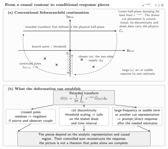
Schematic retarded contour for $e^{-i\omega t}$ and $t>0$, not to scale. On the conventional Schwarzschild sheet shown here, lowering the physical upper-half-plane line crosses specified damped poles and follows the two banks of a negative-imaginary-axis cut. Residues can generate ringdown, threshold discontinuities can generate tails, and the prompt/direct part may be carried by a large-frequency contribution or by a different cut representation. The diagram guides contour deformation without claiming pole completeness; every arc, sheet, orientation, and causal-region assumption still requires proof.

In particular, $t\gt0$ in the schematic does not certify that its large arc vanishes. The exact example required the stronger arrival condition $t\gt d$.

Su and collaborators provide a useful representation-dependent comparison. They split the Schwarzschild Regge–Wheeler kernel into two terms with different large-frequency growth. For $x\gt x'\gt0$ in the intermediate region $x-x'\lt t\lt x+x'$, the direct response can be written using positive- and negative-imaginary-axis cut integrals and a small origin detour. A later-time contour recovers the usual quasinormal-mode and tail pieces Su et al. 2026, arXiv version, § II, pp. 3–4 and Fig. 1; Eq. (30), p. 7 (PDF). Their reconstruction is compared with an independent narrow-Gaussian time-domain evolution Su et al. 2026, arXiv version, § III D, p. 8 and Fig. 6, p. 9 (PDF). The paper is now published; these locators identify the inspected preprint version. This particular Schwarzschild calculation neither proves pole completeness nor establishes the corresponding Kerr decomposition.

A pole expansion can omit a tail or fail before its convergence start time. A local Hadamard construction, conversely, describes nearby singular propagation without enumerating global resonances. These are complementary descriptions. Inverse Transforms and Causal Time-Domain Response develops the contour assumptions needed to assemble them.

Exercises

A tail with its normalization. Suppose $\Delta g(-i\nu)=C\nu^p+O(\nu^{p+1})$ near zero, with $p\gt-1$. Assume also that $e^{-t_0\nu}|\Delta g(-i\nu)|$ is integrable outside every positive neighborhood of zero for some finite $t_0$. Find the leading late-time contribution of the downward cut.

Solution

Split the integral at a small fixed $\nu=\varepsilon$. On the first interval set $y=\nu t$; $p\gt-1$ makes the endpoint integrable. The leading integral is $\Gamma(p+1)t^{-p-1}$, and the local remainder is $O(t^{-p-2})$. The far-cut assumption bounds the second interval by a constant times $e^{-(t-t_0)\varepsilon}$ for sufficiently large $t$. Keeping the east-minus-west prefactor gives

$$G_{\mathrm{cut}}(t) =-\frac{iC\Gamma(p+1)}{2\pi}\,t^{-p-1} +O(t^{-p-2}).$$

The local threshold expansion alone would not justify discarding the far cut. This is the asymptotic of this contribution, not a completeness statement or a claim that all other response components decay faster.

A genuine double pole. Let $\operatorname{Im}\omega_0\lt0$ and

$$H(\omega)=\frac{A+B(\omega-\omega_0)}{(\omega-\omega_0)^2},$$

where $A,B$ are constants. Evaluate its inverse for $t\gt0$, and explain what changes when $A=0$.

Solution

The rational function has no cuts, and its large arc vanishes for $t\gt0$. Differentiate the numerator including the temporal exponential to find the residue $(B-itA)e^{-i\omega_0t}$. Clockwise closure multiplies it by $-i$:

$$H_{\mathrm{ret}}(t)=(-At-iB)e^{-i\omega_0t}, \qquad t\gt0.$$

If $A=0$ and $B\ne0$, the pole is simple and the time-linear term is absent. If both vanish, this entire rational function vanishes. In more general examples full pole cancellation may leave an analytic part with a prompt distributional inverse, so cancellation does not automatically erase the whole response. Finally, a polynomial times a damped exponential still decays at late time; a double pole is not by itself an instability.

References

• Casals, M., and Ottewill, A. C. (2013). “Analytic investigation of the branch cut of the Green function in Schwarzschild space-time.” Physical Review D 87, 064010. DOI. Open PDF, arXiv:1210.0519v1.
• Leaver, E. W. (1986). “Spectral decomposition of the perturbation response of the Schwarzschild geometry.” Physical Review D 34, 384–408. DOI. Open PDF, author version.
• National Institute of Standards and Technology (n.d.). Digital Library of Mathematical Functions, Chapter 10, “Bessel Functions,” §§ 10.9 and 10.17. Integral representations. Large-argument expansions.
• Su, J., Khera, N., Casals, M., Ma, S., Chowdhuri, A., and Yang, H. (2026). “Decomposition of the Schwarzschild Green’s function.” Physical Review D 113, 104013. DOI. Open PDF, arXiv:2601.22015v2.