Geometric-Optics and Eikonal Propagation

Geometric optics is the controlled short-wavelength limit in which a wavefront propagates along rays. For minimally coupled massless test fields, the leading phase satisfies a null Hamilton–Jacobi equation; the next order transports amplitude and polarization along the resulting null geodesics. On a black-hole background this hierarchy explains horizon-directed rays, lensing and focusing, and the dominant large-angular-momentum barrier near unstable photon orbits. It is an asymptotic expansion, not a replacement for the full wave problem near caustics, turning points, boundaries, or wavelengths comparable to curvature scales.

Required background. PDEs and Green Functions for Gravitation supplies principal symbols, characteristics, and asymptotic boundary problems.

Helpful background. Black-Hole Geometry and Mechanics supplies null geodesics and stationary horizons; Formulations of General Relativity supplies characteristic formulations and transport; Frames, Coframes, and Anholonomy supplies screen frames and polarization bases.

Phase surfaces and null rays

Work in a smooth region of a four-dimensional fixed spacetime. Let $\varepsilon\ll1$ be a dimensionless expansion parameter and $S$ a real, dimensionless phase varying on a background scale $\mathcal L$. The physical wavelength must be short compared with the curvature, amplitude and beam variation scales in a regular local frame; a short coordinate wavelength alone is not sufficient. For a massless scalar, write

$$\Phi=\operatorname{Re}\left\{ \left(A_0+\varepsilon A_1+\cdots\right)e^{iS/\varepsilon} \right\}, \qquad k_\mu=\nabla_\mu S,$$

with smooth, possibly complex amplitudes. The actual wave covector and the angular frequency measured by a future-directed unit observer $u^\mu$ are

$$K_\mu=\frac{k_\mu}{\varepsilon}, \qquad \omega_{\rm obs}=-u^\mu K_\mu\gt0, \qquad \lambda_{\rm obs}=\frac{2\pi}{\omega_{\rm obs}}.$$

The inequality chooses a future-directed ray. In a stationary chart, $S=-\mathcal E t+S_{\rm spatial}$ with $\mathcal E\gt0$ gives the positive Killing-frequency mode $e^{-i\omega t}$ with $\omega=\mathcal E/\varepsilon$. Here $\mathcal E$ has inverse-length units; it is not an energy density. The distinction between an order-counting parameter and observer frequency is emphasized by Dolan 2018, §3.1, pp. 6–7, PDF.

The product rule makes the approximation explicit. For any smooth amplitude $a$,

$$e^{-iS/\varepsilon}\Box(ae^{iS/\varepsilon}) =-\frac{k^2}{\varepsilon^2}a +\frac{i}{\varepsilon} \left(2k^\mu\nabla_\mu a+a\nabla_\mu k^\mu\right) +\Box a.$$

The leading nonzero $A_0$ therefore requires the eikonal equation

$$k^\mu k_\mu=0.$$

Because $k_\mu$ is a gradient, $\nabla_\mu k_\nu=\nabla_\nu k_\mu$. Differentiating the eikonal equation therefore gives

$$k^\nu\nabla_\nu k_\mu =\frac12\nabla_\mu(k^\nu k_\nu)=0.$$

The curves $dx^\mu/d\lambda=k^\mu$ are affinely parameterized null geodesics. Their affine normalization is set by $S$; $\lambda$ is not proper time or generally a coordinate distance. A null normal is also tangent to its phase hypersurface, since $k^\mu\nabla_\mu S=0$. Thus these rays generate the null phase surfaces. On a local observer’s spatial slice, their spatial directions are normal to the wavefronts.

For a fixed nonzero field mass in $(\Box-\mu^2)\Phi=0$, the mass enters two orders later, so sufficiently high-frequency rays are still null. If instead the WKB scaling keeps $\varepsilon\mu$ finite by taking $\mu=\bar\mu/\varepsilon$, the leading equation becomes $k^2+\bar\mu^2=0$ and the rays are timelike. Saying that every massive wave follows a null ray therefore suppresses a necessary scale comparison.

For that mass scaling, $\bar\mu$ is constant; a varying effective mass would add a force rather than give geodesic timelike rays.

Amplitude, optical expansion, and caustics

At order $\varepsilon^{-1}$, the scalar equation gives

$$2k^\mu\nabla_\mu A_0+A_0\nabla_\mu k^\mu=0.$$

Multiplying by $\bar A_0$ and adding the conjugate equation gives the positive amplitude-squared conservation law

$$\nabla_\mu(\lvert A_0\rvert^2k^\mu)=0.$$

The two-dimensional screen is the space transverse to a ray after identifying displacements that differ by a multiple of $k^\mu$. Before a caustic, its infinitesimal bundle area $\mathcal A$ satisfies

$$\Theta=\nabla_\mu k^\mu =\frac{d\ln\mathcal A}{d\lambda}, \qquad \frac{d\ln\lvert A_0\rvert}{d\lambda}=-\frac12\Theta, \qquad \lvert A_0\rvert^2\mathcal A=\text{constant}.$$

The logarithmic formula assumes $A_0\ne0$. Our $\Theta$ is the full area expansion; an optical convention using its half-trace would call the expansion $\Theta/2$. The area construction and this convention distinction are given in Dolan 2018, §§4.1.3–4.2.1, pp. 10–11, PDF.

An expanding bundle loses field amplitude, while a focused bundle gains it. For a twist-free congruence, the four-dimensional Raychaudhuri equation is

$$\frac{d\Theta}{d\lambda} =-\frac12\Theta^2-\sigma_{\mu\nu}\sigma^{\mu\nu} -R_{\mu\nu}k^\mu k^\nu.$$

Here $\sigma_{\mu\nu}$ is the symmetric trace-free part of the screen projection of $\nabla_\nu k_\mu$; it describes distortion at fixed area. The twist vanishes because $k=dS$. Curvature can therefore focus the beam directly through the Ricci term or through tidal generation of shear, even though its leading propagation remains null. This is a local transport statement, not by itself a global focusing theorem.

At a caustic, the transverse ray-map determinant vanishes and $\mathcal A\to0$. For nonzero transported flux the leading amplitude diverges, but the finite-wavelength field need not. The ray coordinates have failed. A uniform wave approximation, or matched branches with the appropriate phase information, is needed to pass through the caustic; merely retaining the divergent amplitude is not a solution. A point focus need not create a multibranch region everywhere beyond it. A radial WKB turning point likewise requires a local connection treatment, although neither is necessarily a singularity of the spacetime.

The shared figure makes this distinction visible with a constant-speed flat-space example. Follow the rays through the focus: they continue along straight lines and separate again. If the initial transverse labels are $\mathbf q=(q_1,q_2)$ and the focus is at $x=a\gt0$, the full two-dimensional transverse map is

$$\mathbf y(x,\mathbf q)=(1-x/a)\mathbf q, \qquad J_\perp=\det\frac{\partial\mathbf y}{\partial\mathbf q} =(1-x/a)^2.$$

Away from the focus its inverse is unique. A signed separation in the drawing reverses, but this full determinant is positive on both sides. The initial vertical cross-section is not a wavefront. For each infinitesimal bundle, projecting the vertical section onto a ray-orthogonal screen introduces a raywise constant obliquity factor, so its screen-area ratio follows the same determinant. The foundational geometric-optics page derives this projection factor explicitly.

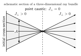
In this constant-speed flat-space model with fixed raywise frequency, $\lvert A_0\rvert^2\mathcal A=\text{constant}$ for an infinitesimal screen on each smooth branch. Focusing raises the leading amplitude, but geometric continuation alone does not fix wave matching through the point caustic. The full transverse determinant $J_\perp$ vanishes only there and is positive on both sides. Schematic section of a three-dimensional bundle, not to scale or a Schwarzschild ray plot.

The conservation law is a useful normalization check: an amplitude $\lvert A_0\rvert\propto\mathcal A^{-1}$ is off by a square root. For radial propagation with $\mathcal A\propto r^2$, it instead gives $\lvert A_0\rvert\propto r^{-1}$. This is not yet a law for the intensity measured by different observers. That additionally depends on frequency, as the Schwarzschild example below demonstrates.

Nor does the transport equation make the wave exact: the unretained $\Box A_0$ generally drives the next amplitude through $2k\cdot\nabla A_1+\Theta A_1=i\Box A_0$. Geometric optics requires this hierarchy to remain ordered over the region and propagation time of interest.

Electromagnetic polarization transport

For source-free Maxwell theory, $F_{\mu\nu}=2\nabla_{[\mu}A_{\nu]}$ and $\nabla_\mu F^{\mu\nu}=0$. In Lorenz gauge these imply

$$\nabla_\mu A^\mu=0, \qquad \Box A_\mu-R_\mu{}^\nu A_\nu=0.$$

The Ricci term is lower order in the short-wavelength expansion, but it is part of the exact operator; see Dolan 2018, §2.2.2, pp. 4–5, Eq. (9), PDF. Take

$$A_\mu=\operatorname{Re}\left\{ (a_\mu+\varepsilon b_\mu+\cdots)e^{iS/\varepsilon} \right\}.$$

The wave equation and leading gauge equation give

$$k^2=0, \qquad k^\mu a_\mu=0.$$

At the next order, the wave and gauge equations give

$$2k^\nu\nabla_\nu a_\mu+\Theta a_\mu=0, \qquad k^\mu b_\mu=i\nabla^\mu a_\mu.$$

The second relation is the next Lorenz constraint: subleading amplitudes are not arbitrary. A residual transformation $A\mapsto A+d\chi$ must satisfy $\Box\chi=0$. Choosing $\chi=\operatorname{Re}\{-i\varepsilon\alpha e^{iS/\varepsilon}+\cdots\}$ changes the leading amplitude by $a_\mu\mapsto a_\mu+\alpha k_\mu$; $\alpha$ itself obeys the leading scalar transport equation. It is not an unrestricted function at every WKB order.

On a patch with nonzero physical amplitude, write $a_\mu=Ae_\mu$ with $A\gt0$ and complex screen polarization satisfying

$$k^\mu e_\mu=0, \qquad \bar e_\mu e^\mu=1, \qquad e_\mu\sim e_\mu+\beta k_\mu.$$

The Hermitian norm is essential: for orthonormal real screen vectors $e_1,e_2$, circular polarization $e=(e_1+i e_2)/\sqrt2$ has $e\cdot e=0$ but $\bar e\cdot e=1$. Splitting the amplitude transport from the vector equation gives $k\cdot\nabla A=-\Theta A/2$ and, on the screen,

$$k^\nu\nabla_\nu e_\mu=0 \quad \text{modulo }k_\mu.$$

Norm and transversality are preserved. A parallel-propagated representative can be chosen along each smooth ray; an arbitrarily rotating observer basis will still show changing components. Comparing emission and reception polarizations requires specifying both physical frames, not erasing that comparison by a coordinate choice. The equivalent field-strength construction is developed in Dolan 2018, §3.2, pp. 7–8, PDF.

With the canonical real-field action $-\frac14\int F_{\mu\nu}F^{\mu\nu}\sqrt{-g}\,d^4x$, the leading Faraday amplitude is $iA(k_\mu e_\nu-k_\nu e_\mu)/\varepsilon$. Inserting it into the stress tensor and averaging the real wave over many cycles gives

$$T_{\mu\nu}=F_{\mu\alpha}F_\nu{}^\alpha -\frac14g_{\mu\nu}F_{\alpha\beta}F^{\alpha\beta}, \qquad \langle T_{\mu\nu}\rangle =\frac{A^2}{2\varepsilon^2}k_\mu k_\nu +O(\varepsilon^{-1}).$$

The factor $1/2$ is the real-wave average, including for a complex polarization normalized as above. $A$ here is a potential amplitude, not the Faraday amplitude used in Dolan’s Eq. (25). For a canonical real massless scalar, the same leading expression holds with $A^2$ replaced by $\lvert A_0\rvert^2$. Its local energy density is therefore $\langle T_{\mu\nu}\rangle u^\mu u^\nu =\lvert A_0\rvert^2\omega_{\rm obs}^2/2$ at leading order. Conservation of this null-fluid stress follows independently from ray geodesy and amplitude transport. Corrections beyond this leading hierarchy, plasma dispersion and nonlinear electrodynamics are outside this vacuum result.

A Schwarzschild beam and its measured flux

Let $m=GM\gt0$, $f=1-2m/r$ and $dr_*/dr=f^{-1}$ in the exterior $r\gt2m$. For an outgoing radial scalar beam, choose

$$S=\mathcal E(r_*-t), \qquad k^\mu=(\mathcal E/f,\mathcal E,0,0), \qquad A_0=C/r,$$

where $\mathcal E\gt0$ and $C$ are constants. Then $\Theta=2\mathcal E/r$, and the transport equation is satisfied. This leading wave is not exact in Schwarzschild: $\Box(C/r)=-2mC/r^4$, which vanishes only in the flat limit or for zero amplitude. The subleading curvature term is a concrete reminder of the approximation being made.

A static observer has $u=f^{-1/2}\partial_t$ and outward unit radial vector $n=f^{1/2}\partial_r$. That observer measures

$$\omega_{\rm obs}=\frac{\mathcal E}{\varepsilon\sqrt f}, \qquad \mathcal F_{\rm loc} =-\langle T_{\mu\nu}\rangle u^\mu n^\nu =\frac{|C|^2\mathcal E^2}{2\varepsilon^2r^2f}.$$

These are leading-order expressions. The conserved quantity for a spherically symmetric beam is the Killing luminosity,

$$\mathscr L=-4\pi r^2\langle T^r{}_t\rangle =4\pi r^2f\,\mathcal F_{\rm loc} =\frac{2\pi|C|^2\mathcal E^2}{\varepsilon^2}.$$

For a small bundle, replace $4\pi$ by its fixed solid angle. The factor $f$ combines the local energy redshift and the clock-rate conversion. Static observers do not exist on the horizon; their divergent measured frequency as $r\to2m$ is not an invariant divergence seen by every observer.

For example, an outward beam compared at $r_i=3m$ and $r_f=6m$ has

$$\frac{|A_{0,f}|}{|A_{0,i}|}=\frac12, \qquad \frac{\omega_{{\rm obs},f}}{\omega_{{\rm obs},i}}=\frac1{\sqrt2}, \qquad \frac{\mathcal F_{{\rm loc},f}}{\mathcal F_{{\rm loc},i}}=\frac18.$$

Area dilution alone would give $1/4$ for amplitude-squared. The additional frequency-squared factor is why the local energy flux instead falls by eight.

Schwarzschild photon sphere from the eikonal barrier

Continue with the same Schwarzschild exterior. For the massless scalar, the exact separated potential and its leading large-$\ell$ part are

$$V_\ell(r)=f\left[\frac{\ell(\ell+1)}{r^2}+\frac{2m}{r^3}\right] =L^2U(r)+f\left(\frac{2m}{r^3}-\frac1{4r^2}\right), \qquad L=\ell+\frac12.$$

Here $U=f/r^2$. Its maximum satisfies

$$\frac{d}{dr}\left(\frac{1-2m/r}{r^2}\right) =-\frac{2}{r^3}+\frac{6m}{r^4}=0,$$

so

$$r_{\mathrm{ph}}=3m=3GM.$$

The ray calculation supplies a separate check and fixes the time used for instability. For an equatorial ray with conserved $\mathcal E=-k_t\gt0$ and $j=k_\phi\gt0$, the null Hamiltonian gives

$$\left(\frac{dr}{d\lambda}\right)^2 =\mathcal E^2-j^2U(r), \qquad \frac{dt}{d\lambda}=\frac{\mathcal E}{f}, \qquad \frac{d\phi}{d\lambda}=\frac{j}{r^2}.$$

Circularity requires $U'=0$ and $j/\mathcal E=1/\sqrt{U(3m)}=3\sqrt3\,m$. Since $U''(3m)=-2/(81m^4)$, a small radial displacement at fixed $\mathcal E,j$ obeys

$$\frac{d^2\delta r}{d\lambda^2} =-\frac{j^2}{2}U''(3m)\,\delta r, \qquad \Lambda_{\rm aff}=\frac{\mathcal E}{\sqrt3\,m}, \qquad \lambda_{\rm ph} =\frac{\Lambda_{\rm aff}}{(dt/d\lambda)_{3m}} =\frac1{3\sqrt3\,m}.$$

$\Lambda_{\rm aff}$ depends on the arbitrary affine normalization; $\lambda_{\rm ph}$ measures the growing branch $\delta r\propto e^{\lambda_{\rm ph}t}$ using Schwarzschild time normalized at infinity. The orbit’s angular rate uses that same time:

$$\Omega_{\mathrm{ph}}=\frac{1}{3\sqrt3\,m}, \qquad \lambda_{\mathrm{ph}}=\frac{1}{3\sqrt3\,m}.$$

The coordinate-time conversion is essential when comparing orbit growth with a frequency-domain decay rate; Cardoso, Miranda, Berti, Witek, and Zanchin 2009, §§II–III, pp. 3–5, Eqs. (19), (27), (34)–(46), PDF derives it and the barrier-WKB connection. Their opposite metric signature does not change these positive rates after translating the conserved quantities; their geometrized mass is our $m=GM$.

For this scalar wave problem, a first-order barrier calculation with ingoing horizon and outgoing infinity conditions gives, for fixed overtone $n$ as $L\to\infty$,

$$\omega_{\ell n} \simeq L\Omega_{\rm ph} -i\left(n+\frac12\right)\lambda_{\rm ph}.$$

The negative imaginary part is damping with the site’s time convention. Geometry alone did not impose those wave boundary conditions or justify the approximation. The derivation, error tests and finite-multipole limits continue in WKB and Geometric-Optics Spectra.

Domain of validity

The eikonal correspondence is not universal. It can fail or require modification for coupled systems whose principal characteristics differ from the metric null cone, for dispersive massive or plasma modes, near degenerate trapping, at finite $\ell$, and with reflecting anti-de Sitter boundaries. Even when a photon orbit controls a leading resonance, excitation amplitudes and completeness do not follow from the orbit alone.

Geometric optics also says nothing by itself about metric backreaction or nonlinear focusing beyond the fixed background. Quantum-state particle interpretation remains separate: a classical WKB ray and positive local frequency do not select a global vacuum in QFT in Curved Spacetime.

Exercises

Focusing is not the whole intensity law. A scalar beam’s screen area decreases by nine without reaching a caustic. Find the amplitude change. If the final observer measures half the initial frequency, by what factor does the leading energy intensity change?

Solution

Conservation of $\lvert A_0\rvert^2\mathcal A$ gives

$$\frac{|A_{0,f}|}{|A_{0,i}|} =\sqrt{\frac{\mathcal A_i}{\mathcal A_f}}=3.$$

The amplitude grows by three, but intensity is proportional to $|A_0|^2\omega_{\rm obs}^2$. Its ratio is therefore $9/4$, not nine. Nine would require equal measured frequencies. Both statements assume the same field normalization and a smooth transported bundle.

A complex polarization can have zero bilinear norm. For $e=(e_1+i e_2)/\sqrt2$ in an orthonormal real screen, calculate $e\cdot e$ and $\bar e\cdot e$. Explain why the first does not signal zero radiation, and why adding $\beta k$ leaves the leading Faraday field unchanged.

Solution

The bilinear contraction is $(1+i^2)/2=0$, whereas the Hermitian contraction is $(1+|i|^2)/2=1$. Physical polarization intensity uses the latter. The gauge addition contributes $k_\mu k_\nu-k_\nu k_\mu=0$ to the leading Faraday amplitude. It also leaves the Hermitian norm unchanged because $k^2=k\cdot e=0$; retaining Lorenz gauge at subsequent orders still requires the residual gauge hierarchy.

Which instability clock? Recover the photon-sphere radius from $U=f/r^2$. What happens to the affine growth exponent and coordinate-time rate if the phase is rescaled by a positive constant? Why does neither calculation establish an exact finite-$\ell$ resonance?

Solution

Differentiating gives $-2/r^3+6m/r^4$, with root $r=3m$ and negative second derivative. Under $S\mapsto cS$ with $c\gt0$, both $\mathcal E$ and $j$ scale by $c$, so $\Lambda_{\rm aff}$ and $dt/d\lambda$ scale by $c$. Their ratio $\lambda_{\rm ph}$ is unchanged. The exact scalar potential also has terms of order $L^0$, and a resonance must satisfy both wave endpoint conditions. The orbit fixes a leading approximation, not the exact finite-$\ell$ frequency, excitation or a complete mode expansion.

References

• Cardoso, Vitor, Alex S. Miranda, Emanuele Berti, Helvi Witek, and Vilson T. Zanchin. “Geodesic Stability, Lyapunov Exponents, and Quasinormal Modes.” Physical Review D 79 (2009): 064016. DOI. Open PDF, arXiv:0812.1806v3.
• Dolan, Sam R. “Geometrical Optics for Scalar, Electromagnetic and Gravitational Waves on Curved Spacetime.” International Journal of Modern Physics D 27, no. 11 (2018): 1843010. DOI. Open PDF, arXiv:1806.08617v1.