WKB and Geometric-Optics Spectra

Barrier-top WKB connects a wave resonance to the height and curvature of a potential maximum. At large angular momentum, that maximum approaches an unstable photon orbit: its orbital frequency sets the leading oscillation rate, and its instability sets the leading damping rate. This page derives that connection for a frequency-independent, single-barrier wave equation with radiative endpoints, then tests its accuracy for Schwarzschild gravitational perturbations. A photon sphere by itself does not determine a general black-hole spectrum.

Required background. PDEs and Green Functions for Gravitation supplies asymptotic waves, turning points, and complex continuation.

Helpful background. Black-Hole Geometry and Mechanics supplies null geodesics; Formulations of General Relativity supplies perturbation variables; Computational Relativity supplies numerical comparison; Black-Hole Perturbation Theory supplies the master potentials.

Resonances near a barrier maximum

Consider a canonically normalized scalar master equation—“scalar” here means one decoupled radial unknown, not necessarily a spin-zero physical field—

$$\frac{d^2X}{dx^2}+[\omega^2-V(x)]X=0, \qquad x=r_*.$$

Assume a real, frequency-independent potential on the real axis with one nondegenerate maximum at $x_0$. The endpoints are short range: for example, $V(x)=O(|x|^{-1-\delta})$ for some $\delta\gt0$ as $x\to\pm\infty$. This supports the plane-wave branches at nonzero real frequency; merely tending to zero is insufficient, since a Coulomb-like tail adds a logarithmic phase. The local expansion also requires enough analyticity to continue through the relevant complex turning-point region. We seek the retarded resonance satisfying

$$X\sim e^{-i\omega x}\quad(x\to-\infty), \qquad X\sim e^{+i\omega x}\quad(x\to+\infty).$$

The first wave travels into the future horizon; the second travels out to infinity. Both travel away from the barrier. These endpoint labels refer to analytic continuation of the scattering solutions, not to a square-integrable eigenfunction: when $\operatorname{Im}\omega\lt0$, the resonant radial profile grows at the ends. See Quasinormal Boundary Conditions and Resonances for this distinction.

Define the peak derivatives and two positive quantities

$$V_k=\left.\frac{d^kV}{dx^k}\right|_{x_0}, \qquad V_1=0,\quad V_2\lt0, \qquad D=\sqrt{-2V_2},\quad N=n+\frac12.$$

Here $n=0,1,\ldots$ labels the low-lying barrier resonances. The turning points solve $\omega^2=V(x)$; the barrier-top approximation concerns the pair close to $x_0$. A single real maximum alone does not guarantee the required global connection to the two endpoint waves.

Why the quadratic barrier gives a complex frequency

Introduce a dimensionless bookkeeping parameter $\epsilon$ and write

$$\left[-\epsilon^2\frac{d^2}{dx^2}+V(x)\right]X=EX.$$

The original equation is recovered with $\epsilon=1$ and $E=\omega^2$. Near the maximum,

$$V(x)=V_0-\beta^2(x-x_0)^2+\cdots, \qquad \beta=\sqrt{-V_2/2}.$$

This is an inverted oscillator. The local outgoing phase is proportional to $\exp[i\beta(x-x_0)^2/(2\epsilon)]$: its phase gradient points right for $x\gt x_0$ and left for $x\lt x_0$. Continue onto the contour

$$x-x_0=e^{i\pi/4}\sqrt{\frac{\epsilon}{\beta}}\,y.$$

That phase becomes $e^{-y^2/2}$, while the differential equation becomes

$$-i\epsilon\beta\left(-\frac{d^2}{dy^2}+y^2\right)X =(E-V_0)X.$$

The decaying oscillator solutions have eigenvalues $2n+1$. Thus

$$E=V_0-i\epsilon N D, \qquad \omega^2_{\mathrm{WKB1}}=V_0-iND.$$

The contour rotation explains the sign and half-integer. It is an auxiliary analytic continuation, not a physical square-integrability condition on real $r_*$. Matching the parabolic-cylinder solutions to the endpoint waves gives the same rule; the original treatment uses the opposite time convention Schutz–Will 1985, Eqs. (3)–(6), pp. L34–L35.

For the positive-frequency branch, choose

$$\operatorname{Re}\omega_{\mathrm{WKB1}}\gt0, \qquad \operatorname{Im}\omega_{\mathrm{WKB1}}\lt0.$$

A negative imaginary part of $\omega^2$ does not select this branch by itself: the other square root grows in time. For a real potential, the negative-frequency damped partner is $-\omega^*$, not $-\omega$.

The formal $\epsilon$ expansion becomes a controlled large-angular-momentum organization when the potential has the form $V=L^2U+O(1)$: divide the wave equation by $L^2$ and identify $\epsilon=1/L$. For a fixed low multipole, setting $\epsilon=1$ provides an approximation to test, not a small-parameter guarantee.

Higher derivatives and WKB orders

Cubic and higher terms describe the departure from the inverted parabola. The complete corrections through third WKB order can be written using

$$q_k=\frac{V_k}{V_2}, \qquad k=3,4,5,6,$$

as

$$\Lambda_2= \frac1D\left[ \frac{q_4}{8}\left(\frac14+N^2\right) -\frac{q_3^2}{288}(7+60N^2) \right],$$ $$\begin{aligned} \Omega_3=\frac1{D^2}\bigg[ &\frac{5q_3^4}{6912}(77+188N^2) -\frac{q_3^2q_4}{384}(51+100N^2)\\ &+\frac{q_4^2}{2304}(67+68N^2) +\frac{q_3q_5}{288}(19+28N^2)\\ &-\frac{q_6}{288}(5+4N^2) \bigg]. \end{aligned}$$

Both $\Lambda_2$ and $\Omega_3$ are real and dimensionless for this real barrier. In particular, $V_k$ has dimensions length$^{-2-k}$ and $D$ has dimensions length$^{-2}$. The three approximations compared below are defined by

$$\begin{aligned} \omega_{\mathrm{WKB1}}^2&=V_0-iND,\\ \omega_{\mathrm{WKB2}}^2&=V_0+D\Lambda_2-iND,\\ \omega_{\mathrm{WKB3}}^2&=V_0+D\Lambda_2-iND(1+\Omega_3). \end{aligned}$$

Take the positive-real, negative-imaginary square root in each case. These are the explicit frequency formulas of Iyer 1987, Eqs. (1.2)–(1.3), p. 3633. The correction symbols in an implicit WKB quantization condition are not interchangeable with these real definitions without translating their factors of $i$.

Why do these orders involve derivatives through fourth and sixth order? Under the rotation, a Taylor term of degree $k$ carries $\epsilon^{k/2}$. The cubic term has zero first-order expectation in an oscillator state, but contributes at second perturbative order, together with the quartic term at first order. The next correction includes sextic, cubic–quintic, quartic–quartic, cubic–cubic–quartic, and four-cubic contributions. The downloadable calculation independently reconstructs these terms using oscillator perturbation theory, retaining intermediate states outside the target state. It does not merely evaluate the same printed polynomial twice.

Higher order is not synonymous with greater accuracy. WKB is generally asymptotic: compare successive orders with an independently converged calculation. Their difference is a useful warning signal, not a guaranteed error bar.

Schwarzschild: the finite-multipole barrier

For axial gravitational perturbations, let $\mu=GM$ denote the gravitational length and use the Regge–Wheeler potential:

$$V_\ell(r)=f(r) \left[\frac{\ell(\ell+1)}{r^2}-\frac{6\mu}{r^3}\right], \qquad f(r)=1-\frac{2\mu}{r}, \qquad \ell\ge2.$$

Frequencies below are dimensionless $w=\mu\omega$. The Schwarzschild $m$ labels are degenerate. An overall constant rescaling of $X$ changes neither the potential nor its frequencies.

Set $k=\ell(\ell+1)$. Since $f\gt0$ outside the horizon, the exterior extremum can be found from $dV/dr=0$. Its radius is

$$\frac{r_0}{\mu} =\frac{3(k+3)+\sqrt{9(k+3)^2-96k}}{2k}.$$

The other quadratic root is not an exterior maximum for $\ell\ge2$. The gravitational quadrupole peak is therefore not at the photon sphere.

Angular label	$r_0/\mu$	Interpretation
$\ell=2$	$3.280776$	appreciable finite-multipole displacement
$\ell=10$	$3.009316$	near the null-orbit maximum
$\ell\to\infty$	$3$	photon-sphere limit

The figure compares the whole normalized barrier, not only its peak position. Inspect the lower, outward-shifted quadrupole curve and the approach of the dashed curve to the dotted limit.

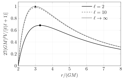
Normalized Schwarzschild axial gravitational barriers approach the null-orbit barrier as $\ell$ increases. The $\ell=2$ maximum is at $3.280776\,GM$; the $\ell=10$ maximum is at $3.009316\,GM$, approaching the photon sphere at $3GM$. The ordinate is $27(GM)^2V/[\ell(\ell+1)]$, with its limiting expression used for $\ell\to\infty$. Curves are quantitative evaluations of the stated potentials, not waveforms or uncertainty estimates.

For the WKB coefficients, differentiate with respect to tortoise distance, not areal radius:

$$\frac{d}{dr_*}=f\frac{d}{dr}, \qquad V_{j+1}(r)=f(r)\frac{dV_j(r)}{dr}.$$

Here the second expression denotes the derivative functions before peak evaluation. Iterate first, substitute the exact algebraic peak last. Substituting $V'(r_0)=0$ into an expression and then differentiating that already-specialized expression discards terms needed at higher orders.

Fundamental-mode comparison

For $n=0$, the complete calculation gives:

Order or reference	$\ell=2$: $GM\omega$	$\ell=10$: $GM\omega$
first WKB	$0.398850-0.088285i$	$2.002323-0.095821i$
second WKB	$0.374350-0.094063i$	$1.996792-0.096086i$
third WKB	$0.373162-0.089217i$	$1.996782-0.095864i$
continued fraction	$0.373672-0.088962i$	$1.996788-0.095864i$

The second-order quadrupole result improves the real part but worsens the imaginary part. Third order improves both relative to first order, but still does not give the reference value. For $\ell=10$, the third-order imaginary parts agree at the displayed precision while the real parts differ in the sixth decimal place. Rounded agreement is not exact equality.

The continued-fraction references are fresh numerical solutions of the same global radial problem, not WKB estimates or values inferred from the table. The method and its boundary interpretation are developed in Frobenius Series and Continued Fractions. Increasing fraction depth and arithmetic precision tests the reference separately from changing WKB order; neither operation proves convergence of the WKB expansion.

Download the Python calculation, pinned requirements, and complete results. In a separate Python environment, install the requirements and run:

python3 wkb-order-comparison.py --output wkb-rerun.json

The finite bundle records peak derivatives, all three orders, oscillator checks, continued-fraction depth and precision comparisons, residuals, and rejected wrong-sign or wrong-derivative controls. It covers only the two stated fundamental modes; it is not a general-purpose high-overtone solver.

The photon orbit and its instability rate

To identify exactly which geometric rates enter, consider a static spherical exterior

$$ds^2=-f(r)\,dt^2+\frac{dr^2}{g(r)}+r^2d\Omega^2, \qquad \frac{dr_*}{dr}=\frac1{\sqrt{f(r)g(r)}}.$$

Assume $f,g\gt0$ in the exterior and an asymptotically flat normalization $f\to1$, so $t$ is the clock of a stationary observer at infinity. The following null-geodesic calculation is kinematic; identifying its result with a wave spectrum additionally requires the wave equation and endpoint assumptions below.

For an equatorial null geodesic with affine parameter $\sigma$, conserved energy $\mathcal E=f\,dt/d\sigma$, angular momentum $\mathcal J=r^2d\phi/d\sigma$, and impact parameter $b=\mathcal J/\mathcal E$, define $U=f/r^2$. The null constraint gives

$$\left(\frac{dr}{dt}\right)^2 =fg(1-b^2U), \qquad \left(\frac{dr_*}{dt}\right)^2=1-b^2U.$$

A circular orbit at $r_c$ satisfies

$$U'(r_c)=0,\qquad b_c^2=\frac1{U_c}, \qquad \Omega_c=\left|\frac{d\phi}{dt}\right|_c=\sqrt{U_c}.$$

Primes on $U(r)$ here denote areal-radius derivatives. For an unstable orbit, $U''(r_c)\lt0$. Expanding about it in $\delta x=r_*-r_{*c}$ yields

$$\left(\frac{d\delta x}{dt}\right)^2 =\lambda_c^2\delta x^2+O(\delta x^3), \qquad \lambda_c^2=-\frac{U''_{*c}}{2U_c} =-\frac{f_cg_c\,U''(r_c)}{2U_c}.$$

Thus a departing radial perturbation grows as $e^{\lambda_c t}$. The rate is measured in coordinate time $t$, not in an arbitrarily rescaled null affine parameter. The factor $g_c$ shows why orbital radius and frequency alone do not determine instability. These are the translated static-spherical rates in Cardoso et al. 2009, Eqs. (19), (22), (35), (37), (40)–(41), preprint pp. 3–4, PDF.

Now suppose the actual decoupled wave potential admits

$$V_\ell=L^2U+O(1), \qquad L=\ell+\frac12, \qquad L\to\infty,\quad n\ \text{fixed},$$

with a smooth expansion near the unique nondegenerate maximum and the radiative endpoint connection already specified. The peak height is $L^2U_c+O(1)$ and its second tortoise derivative is $L^2U''_{*c}+O(1)$. Inserting these into the leading barrier rule and taking the positive-frequency square root gives

$$\omega_{\ell n}=L\Omega_c-iN\lambda_c+O(L^{-1}).$$

The orbital phase determines the leading real part; escape from the unstable orbit determines the leading damping. This is the eikonal correspondence, not an independent quantization of a material photon orbit Cardoso et al. 2009, § III C and Eq. (46), preprint pp. 4–5, PDF. The $L=\ell+1/2$ refinement here follows from the stated four-dimensional potential expansion, since $\ell(\ell+1)=L^2-1/4$; it should not be inserted into an arbitrary field equation without checking that expansion.

For Schwarzschild, $f=g=1-2\mu/r$ gives

$$r_c=3\mu,\qquad U_c=\frac1{27\mu^2},\qquad U''_{*c}=-\frac2{729\mu^4}, \qquad \Omega_c=\lambda_c=\frac1{3\sqrt3\,\mu}.$$

Consequently,

$$GM\omega_{\ell n} =\frac{\ell+\tfrac12-i(n+\tfrac12)}{3\sqrt3} +O(\ell^{-1}).$$

This formula discards finite-multipole terms retained by WKB applied to the full Regge–Wheeler potential. It is therefore less accurate than the first-order WKB row at $\ell=2$; the two approximations should not be called the same numerical calculation.

An exactly solvable barrier: Pöschl–Teller

A useful independent check is

$$V(x)=V_0\,\operatorname{sech}^2(\alpha x), \qquad \alpha\gt0,\quad V_0\gt\frac{\alpha^2}{4},$$

with the same two outgoing-from-the-barrier endpoint conditions. The origin has been placed at the maximum. The stated height condition restricts this discussion to the oscillatory resonance pair, away from coincident or purely imaginary cases.

Set

$$z=\frac{1+\tanh(\alpha x)}2,\qquad X=z^p(1-z)^pF(z),\qquad p=-\frac{i\omega}{2\alpha}.$$

The powers supply the desired left ingoing and right outgoing behavior. Since $dz/dx=2\alpha z(1-z)$, direct substitution gives

$$z(1-z)F''+[C-(A+B+1)z]F'-ABF=0,$$

where

$$\begin{aligned} A&=\frac12-\frac{i\omega}{\alpha}+\nu,& B&=\frac12-\frac{i\omega}{\alpha}-\nu,\\ C&=1-\frac{i\omega}{\alpha},& \nu&=\sqrt{\frac14-\frac{V_0}{\alpha^2}}. \end{aligned}$$

Choose $F={}_2F_1(A,B;C;z)$ at the left endpoint. Its connection formula at $z=1$ contains a right-incoming coefficient proportional to

$$C_{\mathrm{in}} =\frac{\Gamma(1-i\omega/\alpha)\,\Gamma(-i\omega/\alpha)} {\Gamma(A)\,\Gamma(B)}.$$

Because the gamma function has no zeros, this coefficient vanishes when $A=-n$ or $B=-n$, provided no numerator pole cancels that zero. In the strictly oscillatory regime specified above there is no such cancellation at these roots. Therefore

$$\omega_n^\pm =\pm\sqrt{V_0-\frac{\alpha^2}{4}} -i\alpha\left(n+\frac12\right).$$

This independently reproduces the translated exact solution of Ferrari–Mashhoon 1984, Eqs. (24)–(27), p. 298, and Appendix A, Eqs. (A1)–(A7), p. 302. Their time convention has the opposite sign. Extending to the critical or weak barrier requires a separate treatment of coincident connection-function poles; the present check does not declare that all nonoscillatory resonances are absent.

At the peak,

$$V_2=-2V_0\alpha^2,\quad V_3=V_5=0,\quad V_4=16V_0\alpha^4,\quad V_6=-272V_0\alpha^6.$$

Substitution into the WKB corrections gives

$$D\Lambda_2=-\alpha^2\left(N^2+\frac14\right), \qquad \Omega_3=-\frac{\alpha^2}{8V_0}.$$

Indeed, the exact positive-branch frequency squared is

$$(\omega_n^+)^2 =V_0-\alpha^2\left(N^2+\frac14\right) -2iN\alpha\sqrt{V_0-\frac{\alpha^2}{4}}.$$

Expanding the last square root at fixed $n$ for $\alpha/\sqrt{V_0}\ll1$ reproduces the third-order expression. This tests the even-derivative terms independently; the separate oscillator calculation tests the odd-derivative terms that vanish for this symmetric barrier.

For a reference length $a_0$, choose $V_0a_0^2=1$, $\alpha a_0=0.2$, and $n=0$. The exact root is

$$a_0\omega_0^+=0.99498744-0.10000000i,$$

whereas the leading parabolic rule gives

$$a_0\omega_{\mathrm{WKB1}} =\sqrt{1-0.2i} =1.00493878-0.09950855i.$$

First-order WKB is not exact even for this smooth single barrier. Conversely, an exact result for the Pöschl–Teller model is not an exact Schwarzschild result: its exponentially decaying outer potential does not reproduce the long-range Schwarzschild threshold structure or power-law tail.

Limits of geometric optics

Low multipoles and high overtones. Small $\ell$ leaves no large-angular-momentum control; increasing $n$ moves the relevant turning points farther from the peak. The assumption here is fixed $n$ as $\ell$ grows, not arbitrary $n$ at any multipole.

Several extrema or a well. Additional turning points create trapping, tunneling, and different connection paths. A local Taylor expansion at one maximum can miss entire mode families and small splittings.

Frequency dependence or coupling. Kerr separation couples the angular eigenvalue to $\omega$; a frequency-dependent radial equation requires a consistent implicit solve. Coupled perturbations or different characteristic cones need not share the background metric’s light-ring formula.

Different outer conditions. A reflecting AdS boundary or a massive-field threshold changes the global resonance problem even if local photon-orbit data look similar. The AdS failure is explicitly discussed in Cardoso et al. 2009, Appendix C, preprint p. 12, PDF.

Use WKB for geometric understanding and economical low-overtone estimates, then compare with a converged global method when accuracy matters. Spectral Collocation and Direct Eigenvalue Methods supplies another such route. Source excitation and detector inference are different questions, outside this page’s scope.

Exercises

Compare the geometric and finite-multipole estimates

Evaluate the Schwarzschild eikonal formula for $n=0$ at $\ell=2$ and $\ell=10$. Compare its real part with the continued-fraction table. Why does using the full potential in first-order WKB improve the quadrupole estimate?

Solution

The eikonal predictions are

$$GM\omega_{20}\simeq0.481125-0.096225i,\qquad GM\omega_{10,0}\simeq2.020726-0.096225i.$$

Their real parts are approximately $28.8\%$ and $1.20\%$ above the corresponding continued-fraction values. The full axial potential includes the negative $6GM/r^3$ term, which is subleading at large $\ell$ but significant at $\ell=2$. It changes both height and curvature, and shifts the quadrupole peak to $3.280776GM$. Keeping those finite-multipole effects gives the first-order WKB value $0.398850-0.088285i$, but does not repair the remaining higher-derivative approximation.

Keep the orbit but change its instability

As a kinematic metric comparison, hold $f=1-2\mu/r$ fixed but choose

$$g=f\left[1+\eta\left(\frac{3\mu}{r}\right)^2\right], \qquad \eta\gt0.$$

No vacuum Einstein solution is being asserted. What happens to $r_c$, $\Omega_c$, and $\lambda_c$? What additional information is needed before predicting a wave spectrum?

Solution

The function $U=f/r^2$ is unchanged, so $r_c=3\mu$ and $\Omega_c=1/(3\sqrt3\mu)$. At the orbit, $g_c$ is multiplied by $1+\eta$, giving

$$\lambda_c=\frac{\sqrt{1+\eta}}{3\sqrt3\,\mu}.$$

Thus equal orbital radius and angular frequency do not imply equal damping. One must still derive the actual decoupled wave equation, show that its leading potential is $L^2U$, and check the radiative endpoints and one-barrier connection. The metric calculation alone does not establish those facts for a chosen matter or gravity theory.

Test the correction signs on a symmetric barrier

Use the Pöschl–Teller derivatives above to recover $D\Lambda_2$ and $\Omega_3$. Which coefficient terms remain untested by this example?

Solution

The nonzero ratios are $q_4=-8\alpha^2$ and $q_6=136\alpha^4$. Thus

$$D\Lambda_2=-\alpha^2\left(N^2+\frac14\right),$$

and

$$\Omega_3 =\frac{\alpha^2}{4V_0} \left[\frac{67+68N^2}{36} -\frac{17(5+4N^2)}{36}\right] =-\frac{\alpha^2}{8V_0}.$$

All $N^2$ terms in the last bracket cancel. The terms involving $q_3$ or $q_5$ vanish before evaluation, so this check cannot validate their coefficients. A nonsymmetric barrier or independent general oscillator calculation is needed.

References

• Cardoso, V., Miranda, A. S., Berti, E., Witek, H., and Zanchin, V. T. (2009). “Geodesic stability, Lyapunov exponents, and quasinormal modes.” Physical Review D 79, 064016. DOI. Open PDF, arXiv:0812.1806v3; page locators above refer to this preprint.
• Ferrari, V., and Mashhoon, B. (1984). “New approach to the quasinormal modes of a black hole.” Physical Review D 30, 295–304. DOI. Open PDF.
• Iyer, S. (1987). “Black-hole normal modes: A WKB approach. II. Schwarzschild black holes.” Physical Review D 35, 3632–3636. DOI. Open PDF.
• Schutz, B. F., and Will, C. M. (1985). “Black hole normal modes: A semianalytic approach.” The Astrophysical Journal Letters 291, L33–L36. DOI. Open PDF.