The Eikonal and Geometric-Optics Limits

Guiding question: What small parameter turns a wave equation into ray dynamics?

When the wavelength is much shorter than every scale on which the medium and wave envelope vary, a rapidly changing phase obeys a Hamilton–Jacobi equation. Its characteristics are rays, while the next asymptotic order transports amplitude along ray tubes. The approximation fails where that scale separation is lost, especially at caustics and turning points.

Required background. Ordinary Differential Equations provides initial-value problems, linearization, and asymptotic solution methods; Classical Field Theory provides field actions, Euler–Lagrange equations, and gauge redundancy. Helpful background. Calculus and Linear Algebra provides multivariable differentiation, linear maps, inner products, and basis changes; Partial Differential Equations and Green Functions provides characteristics, boundary data, distributions, and Green-function methods.

Rays and transport

The parameter is

$$\varepsilon=\frac{\lambda}{L}\ll1,$$

where $\lambda=2\pi/|\mathbf k_{\rm phys}|$ is the local wavelength and $L$ is the shortest scale on which the background, amplitude, wavefront curvature, or apparatus changes appreciably. The eikonal equation is the leading term of an expansion in $\varepsilon$; rays are its characteristics.

Consider

$$\partial_t^2\psi-\boldsymbol\nabla\mathbin{\cdot} \left[v^2(\mathbf x)\boldsymbol\nabla\psi\right]=0,$$

where $v(\mathbf x)\gt0$ varies on scale $L$. Use

$$\psi=\operatorname{Re}\left\{ A(t,\mathbf x)e^{iS(t,\mathbf x)/\varepsilon} \right\}.$$

Because the operator is real, work with the complex expression and take its real part at the end. If $P=\partial_t^2-\boldsymbol\nabla\mathbin{\cdot}(v^2\boldsymbol\nabla)$, direct substitution gives

$$\begin{aligned} e^{-iS/\varepsilon}P\left(Ae^{iS/\varepsilon}\right) ={}&\frac{A}{\varepsilon^2} \left[-S_t^2+v^2|\boldsymbol\nabla S|^2\right]\\ &+\frac{i}{\varepsilon}\left[ 2S_tA_t+A S_{tt} -2v^2\boldsymbol\nabla S\mathbin{\cdot}\boldsymbol\nabla A -A\boldsymbol\nabla\mathbin{\cdot}(v^2\boldsymbol\nabla S) \right]\\ &+A_{tt}-\boldsymbol\nabla\mathbin{\cdot}(v^2\boldsymbol\nabla A). \end{aligned}$$

Each derivative of the phase brings a factor $\varepsilon^{-1}$. The leading $\varepsilon^{-2}$ coefficient gives

$$\boxed{(\partial_tS)^2-v^2|\boldsymbol\nabla S|^2=0.}$$

This is the eikonal, or local dispersion, equation. For $S=-\omega t+W(\mathbf x)$ with $\omega\gt0$ and refractive index $n=1/v$,

$$|\boldsymbol\nabla W|=n\omega.$$

Rosales performs this expansion explicitly in Rosales 2023, §7.1.2, pp. 40–41 (official PDF).

Define the scaled wave covector by

$$k_\mu=\partial_\mu S, \qquad \omega=-\partial_tS, \qquad \mathbf k=\boldsymbol\nabla S.$$

Because the phase is $S/\varepsilon$, the physical frequency and wave vector are $\omega/\varepsilon$ and $\mathbf k/\varepsilon$. Their common rescaling changes the ray parameter but not the ray path.

The eikonal equation is a Hamilton–Jacobi equation for

$$H(x,k)=\frac12\left(-\omega^2+v^2|\mathbf k|^2\right)=0.$$

Hamilton’s equations propagate $(x,k)$ along rays. For the covariant formulas below, specialize to flat vacuum with $v=1$. Then $k_\mu=\partial_\mu S$ is null. Since phase gradients commute,

$$k^\nu\partial_\nu k_\mu =\frac12\partial_\mu(k^\nu k_\nu)=0,$$

so the rays are straight null lines.

At the next order, the constant-speed scalar amplitude obeys

$$\boxed{2k^\mu\partial_\mu A +A\,\partial_\mu k^\mu=0,}$$

and therefore

$$\boxed{\partial_\mu\left(|A|^2k^\mu\right)=0.}$$

The second equation follows by combining the complex transport equation with its conjugate. It conserves leading wave action through a ray tube. At constant speed and fixed raywise frequency in a homogeneous medium, the same area dilution also governs energy flux. Narrowing an infinitesimal ray tube raises $|A|$. The ray and ray-tube construction is developed in Rosales 2023, §7.1.3, pp. 41–43 (official PDF).

The figure makes the limit visible in a constant-speed flat-space model. Track the area as the rays focus: transport predicts growing amplitude until the ray map loses invertibility. The vertical initial cross-section is not a wavefront: the tilted rays are not normal to it.

To specify the geometry, let $x$ run along the central ray, put the focus at $x=a\gt0$, and label rays by their initial transverse position $\mathbf q=(q_1,q_2)$. The full transverse map and its determinant are

$$\mathbf y(x,\mathbf q)=(1-x/a)\mathbf q, \qquad J_\perp=\det\frac{\partial\mathbf y}{\partial\mathbf q} =(1-x/a)^2.$$

For $x\ne a$, the inverse $\mathbf q=\mathbf y/(1-x/a)$ is unique. Only at the focus do all labels coincide. The signed separation visible in this two-dimensional drawing reverses after the focus, but the full transverse determinant is positive on both sides. This point focus does not create a permanent multibranch region.

The area $\mathcal A$ means an infinitesimal screen orthogonal to a ray, not the whole vertical cut. Projecting that cut onto the screen contributes the obliquity factor $a/\sqrt{a^2+|\mathbf q|^2}$, which is constant along each straight ray. Hence the screen-area ratio follows $J_\perp$.

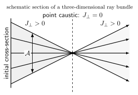
In this constant-speed flat-space model, $|A|^2\mathcal A=\text{constant}$ for an infinitesimal screen on each smooth branch, so focusing raises the leading amplitude. The full transverse determinant $J_\perp$ vanishes only at the point focus and is positive on both sides. Geometric continuation alone does not determine wave matching through the caustic. Schematic section of a three-dimensional bundle, not to scale or a Schwarzschild ray plot.

For electromagnetism, impose Lorenz gauge and write the potential as

$$\mathcal A_\mu=a_\mu e^{iS/\varepsilon}.$$

The leading Maxwell and gauge equations give

$$k^2=0, \qquad k^\mu a_\mu=0,$$

and the next order gives, in flat vacuum,

$$2k^\nu\partial_\nu a_\mu +(\partial_\nu k^\nu)a_\mu=0.$$

After separating the scalar magnitude, the normalized transverse polarization is transported along the ray. A residual change $a_\mu\mapsto a_\mu+\alpha k_\mu$ changes the potential representative but not the leading field strength. The plane-wave transversality and two physical vacuum polarizations are reviewed in Tong 2015, §4.3.2, pp. 87–88 (official PDF); the transport equation above follows from the same WKB expansion as the scalar equation.

Domain of validity

Geometric optics fails near caustics, where neighboring rays cross and nonzero transported flux gives a divergent leading amplitude; the finite-wavelength field need not diverge, and a uniform wave approximation or suitable branch matching is required. It also fails near turning points, sharp interfaces on the scale $\lambda$, apertures comparable to $\lambda$, and polarization-mode degeneracies. Higher-order terms can describe gradual corrections but cannot repair a nonuniform expansion at a caustic. The ray solution’s singular amplitude denominator appears in Rosales 2023, §7.1.6, pp. 46–47 (official PDF), while Airy uniformization and its application to caustics appear in Rosales 2023, §3.3, pp. 20–23 (official PDF).

Ray velocity here follows the high-frequency local dispersion relation. It should not be confused with the group velocity of an arbitrary broad packet or with the large-distance radiation-zone approximation. One can be far from a source without having $\lambda/L\ll1$, and one can have excellent geometric optics close to no localized source at all.

Operationally, interferometric phase measurements reconstruct $S$; normals to equal-phase surfaces give $\mathbf k$. Intensity across a detector array tests the ray-tube transport law.

Transfer task: spherical spreading

In vacuum, take the positive-frequency outgoing phase $S=r-t$. Use amplitude transport to determine the leading radial dependence of $A(r)$.

Solution

The wave covector is null, and rays are radial. Integrate

$$\partial_\mu\left(|A|^2k^\mu\right)=0$$

over a thin ray tube subtending solid angle $d\Omega$. Its cross-sectional area is $r^2d\Omega$, so conservation gives

$$r^2|A|^2=\text{constant}.$$

Hence

$$\boxed{|A(r)|\propto\frac1r.}$$

The result holds away from the origin and before boundaries or focusing intervene. It is an amplitude statement; energy flux scales as $|A|^2\propto r^{-2}$.

Multipole Expansion and Radiation Zones next derives which compact-source moments supply that outgoing $1/r$ field.

References

• R. R. Rosales, Lecture Topics for MIT 18.376, Massachusetts Institute of Technology, 2023, §3.3, pp. 20–23, §§7.1.2–7.1.3, pp. 40–43, and §7.1.6, pp. 46–47 (official PDF).
• David Tong, Lectures on Electromagnetism, University of Cambridge, 2015, §§4.3.1–4.3.2, pp. 84–88 (official PDF).