Plebański–Demiański and the Type-D Electrovacuum Family

Introduced in its canonical form by Plebański and Demiański 1976, the Plebański–Demiański family is a local synthesis of four-dimensional vacuum and aligned non-null Einstein–Maxwell solutions with cosmological constant. Its generic regular members are Petrov type D, and controlled limits also reach nonexpanding Kundt solutions and constant-curvature products. The compact canonical formula is powerful precisely because its coordinates and polynomial coefficients are not yet tied to one black-hole interpretation: mass, acceleration, rotation, NUT charge, and electromagnetic flux acquire those meanings only after a branch, domain, Killing normalization, and angular period have been fixed.

Required background. Frames, Coframes, and Anholonomy supplies principal tetrads and algebraic alignment.

Helpful background. The Einstein Equation supplies Einstein–Maxwell–$\Lambda$ dynamics; The Riemann Curvature Tensor supports type-D and scalar checks; Exact Solutions of Einstein’s Equations supplies family-identification discipline; Causality and Global Structure supplies domain qualifications; Killing Fields and Isometry Groups supplies the two commuting symmetries.

The canonical expanding chart

The displayed chart covers the branch with expanding repeated principal null congruences and non-null two-dimensional Killing orbits. It does not include the separate type-D class with null Killing-group orbits, nor electrovacua in which only one Maxwell principal null direction is aligned. These scope boundaries are explicit in Griffiths and Podolský 2006, §§ 1–2, printed pp. 3–5, Open PDF.

The coordinates $\tau$ and $\sigma$ follow the two commuting Killing fields. The coordinates $p$ and $q$ label their orbits; they become angular-like and radial-like only after a branch-specific transformation. Define

$$\Omega=\frac{1}{1-pq}, \qquad \rho^2=p^2+q^2.$$

A standard $(-,+,+,+)$ representation is

$$\begin{aligned} ds^2=\Omega^2\Bigg[{} &\rho^2\left(\frac{dp^2}{P(p)}+\frac{dq^2}{Q(q)}\right)\\ &+\frac{P(p)}{\rho^2}(d\tau+q^2d\sigma)^2 -\frac{Q(q)}{\rho^2}(d\tau-p^2d\sigma)^2 \Bigg], \end{aligned}$$

where

$$P(p)=k+2np-\epsilon p^2+2mp^3 -\left(k+e^2+g^2+\frac{\Lambda}{3}\right)p^4,$$ $$Q(q)=k+e^2+g^2-2mq+\epsilon q^2-2nq^3 -\left(k+\frac{\Lambda}{3}\right)q^4.$$

This is the signature-translated form of Griffiths and Podolský 2006, § 2.1, printed pp. 4–5, Eqs. (1)–(2), Open PDF, and it agrees directly with Frolov, Krtouš, and Kubizňák 2017, § 3.9, printed p. 68, Eqs. (3.126)–(3.128), Open PDF under $y=p$, $r=q$, and $\psi=-\sigma$.

Coordinate and signature checks

Introduce the Killing one-forms

$$u=d\tau+q^2d\sigma, \qquad v=d\tau-p^2d\sigma.$$

The metric is diagonal in $(dp, dq, u, v)$, while

$$u\wedge v=-\rho^2\,d\tau\wedge d\sigma.$$

Therefore

$$\det g\big|_{\{\partial_\tau,\partial_\sigma\}} =-\Omega^4P(p)Q(q),$$

and the full determinant is

$$\det g=-\Omega^8\rho^4 =-\frac{(p^2+q^2)^2}{(1-pq)^8}, \qquad \sqrt{-g}=\Omega^4\rho^2.$$

On an open cell with $P,Q\ne0$, $\rho^2>0$, and finite $\Omega$, the declared Lorentzian branch requires $P>0$. Then:

• If $Q>0$, both $p$ and $q$ directions are spacelike and the Killing two-plane has one negative eigenvalue. The cell is stationary.
• If $Q<0$, the Killing two-plane is positive definite and $q$ supplies the only negative direction. The cell is dynamical.

A root of $Q$ is consequently only a candidate Killing horizon until its null generator and extension are checked. A root of $P$ may mark an axis or another coordinate boundary, but its regularity depends on the angular identification. After translating their displayed metric to this page’s signature, the sentence immediately below Eq. (2) of Griffiths and Podolský 2006, § 2.1, printed p. 5, Open PDF interchanges the two $Q$-sign labels; the diagonal coframe and determinants above provide the direct check.

The locus $\rho^2=0$ is excluded from this chart. It is a curvature singularity when it lies in the chosen domain and at least one of $m,n,e,g$ is nonzero: the Newman–Penrose Ricci component behaves as $\Phi_{11}\sim(e^2+g^2)/\rho^4$, while the vacuum Coulomb Weyl scalar behaves as $\lvert\Psi_2\rvert\sim\rho^{-3}$ when $m$ or $n$ is nonzero. If $m=n=e=g=0$, however, the solution is locally flat or constant-curvature and $\rho=0$ is only a removable coordinate degeneration. These checks follow from Griffiths and Podolský 2006, § 2.2, printed p. 6, Eqs. (9)–(10), Open PDF.

Maxwell normalization and algebraic type

Use the geometrized Maxwell potential $\mathcal A=\sqrt G\,A_{\rm G}$, where $A_{\rm G}$ is the Gaussian potential, and set $\mathcal F=d\mathcal A$. Equivalently, $\mathcal A=\sqrt{4\pi G}\,A_{\rm R}$ in rationalized units. The field equations are

$$d\mathcal F=0, \qquad d({}^{\star}\mathcal F)=0,$$ $$G_{\mu\nu}+\Lambda g_{\mu\nu} =2\left( \mathcal F_{\mu\alpha}\mathcal F_\nu{}^\alpha -\frac14g_{\mu\nu}\mathcal F_{\alpha\beta}\mathcal F^{\alpha\beta} \right).$$

Choose $d\tau\wedge dq\wedge dp\wedge d\sigma$ to be positively oriented and define the left Hodge dual on the two-form index pair by

$$({}^{\star}\mathcal F)_{\mu\nu} =\frac12\varepsilon_{\mu\nu}{}^{\rho\sigma}\mathcal F_{\rho\sigma}.$$

A site-compatible signed dyonic potential is

$$\mathcal A=-\frac{eq}{\rho^2}(d\tau-p^2d\sigma) +\frac{gp}{\rho^2}(d\tau+q^2d\sigma).$$

When $g\ne0$, this potential is patch-local: regular north- and south-axis gauges differ by a gauge transformation even though the field strength $\mathcal F$ is globally defined away from magnetic sources.

Under $p=a\cos\theta$, $q=r$, $\sigma=-\phi/a$, and $\tau=t-a\phi$, this becomes the dyonic Kerr–Newman potential used elsewhere in this volume. For $a\ne0$ and $0<\theta<\pi$, the orientation Jacobian is $\sin\theta>0$; the axes are coordinate degeneracies of this map. Relative to Frolov, Krtouš, and Kubizňák 2017, § 3.9, printed p. 68, Eq. (3.126), Open PDF, this convention keeps their electric sign and uses $g_{\rm Frolov}=-g$. That is a parameter translation, not a gauge transformation. Multiplying the entire potential by $-1$ would reverse both charges while leaving the stress tensor unchanged.

Let $S$ be an outward-oriented closed two-surface enclosing the source, with the axial orbit normalized to period $2\pi$. In the geometrized convention above, the signed fluxes are

$$e=\frac{1}{4\pi}\int_S{}^{\star}\mathcal F, \qquad g=\frac{1}{4\pi}\int_S\mathcal F.$$

For example, in the Kerr–Newman chart at large $r$, the induced orientation is $d\theta\wedge d\phi$ and the leading fields give ${}^{\star}\mathcal F=e\sin\theta\,d\theta\wedge d\phi$ and $\mathcal F=g\sin\theta\,d\theta\wedge d\phi$. In Gaussian and rationalized conventions, respectively,

$$\begin{aligned} Q_{e,{\rm G}}&=\frac{1}{4\pi}\int_S{}^{\star}F_{\rm G}, &Q_{m,{\rm G}}&=\frac{1}{4\pi}\int_S F_{\rm G},\\ Q_{e,{\rm R}}&=\int_S{}^{\star}F_{\rm R}, &Q_{m,{\rm R}}&=\int_S F_{\rm R}. \end{aligned}$$

Consequently, only after the surface and angular normalization have been fixed may the parameters be identified as

$$\begin{aligned} e&=\sqrt G\,Q_{e,{\rm G}} =\sqrt{\frac{G}{4\pi}}\,Q_{e,{\rm R}},\\ g&=\sqrt G\,Q_{m,{\rm G}} =\sqrt{\frac{G}{4\pi}}\,Q_{m,{\rm R}}. \end{aligned}$$

Before that normalization, $e$ and $g$ remain scale- and period-dependent metric parameters. The complete Gaussian-to-rationalized translation is summarized on Units and Dimensional Conventions.

In a principal tetrad, the Maxwell field has only its Coulomb component and every Weyl scalar except $\Psi_2$ vanishes Griffiths and Podolský 2006, § 2.2, printed p. 6, Eqs. (7)–(10), Open PDF. A regular point is Petrov type D when $\Psi_2\ne0$ and type O when $\Psi_2=0$. Thus “the type-D family” includes conformally flat boundary cases, but they must not themselves be labeled type D.

Exposing acceleration and twist scales

The original hatted form has seven arbitrary parameters $(\hat m,\hat n,\hat e,\hat g,\hat\epsilon,\hat k,\Lambda)$. They encode seven essential degrees of freedom, although most are not yet physical charges. A useful enlarged representation displays nine symbols $(m,n,e,g,\epsilon,k,\Lambda,\alpha,\omega)$ with two scale freedoms; it still describes seven essential parameters Griffiths and Podolský 2006, §§ 2.1–2.2, printed pp. 4–6, Open PDF. This distinction corrects the tempting but false statement that the original seven constants are reduced to five by scaling.

For positive scale choices $\alpha$ and $\omega$, the invertible rescaling is

$$\begin{aligned} \hat p&=\sqrt{\alpha\omega}\,p, &\hat q&=\sqrt{\frac{\alpha}{\omega}}\,r,\\ \hat\sigma&=\sqrt{\frac{\omega}{\alpha^3}}\,\sigma, &\hat\tau&=\sqrt{\frac{\omega}{\alpha}}\,\tau,\\ \hat m+i\hat n&=\left(\frac{\alpha}{\omega}\right)^{3/2}(m+in), &\hat e+i\hat g&=\frac{\alpha}{\omega}(e+ig),\\ \hat\epsilon&=\frac{\alpha}{\omega}\epsilon, &\hat k&=\alpha^2k, \qquad \hat\Lambda=\Lambda. \end{aligned}$$

It obeys $1-\hat p\hat q=1-\alpha pr$. With

$$\varrho^2=r^2+\omega^2p^2, \qquad \Omega_\alpha=\frac{1}{1-\alpha pr},$$

the transformed metric is

$$\begin{aligned} ds^2=\Omega_\alpha^2\Bigg[{} &\varrho^2\left(\frac{dp^2}{P_\alpha}+ \frac{dr^2}{Q_\alpha}\right)\\ &+\frac{P_\alpha}{\varrho^2}(\omega d\tau+r^2d\sigma)^2 -\frac{Q_\alpha}{\varrho^2}(d\tau-\omega p^2d\sigma)^2 \Bigg], \end{aligned}$$

where

$$\begin{aligned} P_\alpha(p)={}&k+2\frac n\omega p-\epsilon p^2+2\alpha mp^3\\ &-\left[ \alpha^2(\omega^2k+e^2+g^2)+\frac{\omega^2\Lambda}{3} \right]p^4, \end{aligned}$$ $$\begin{aligned} Q_\alpha(r)={}&\omega^2k+e^2+g^2-2mr+\epsilon r^2 -2\alpha\frac n\omega r^3\\ &-\left(\alpha^2k+\frac{\Lambda}{3}\right)r^4. \end{aligned}$$

These are Griffiths and Podolský 2006, § 2.2, printed pp. 5–6, Eqs. (3)–(6), Open PDF. The map itself requires nonzero scales. Limits such as $\alpha\to0$ or $\omega\to0$ must first be taken in the finite transformed metric and functions, with the necessary parameter ratios held fixed.

The root-adapted black-hole branch

For an angular polynomial with two distinct roots, an affine change makes those roots $x=\pm1$ and separates a Kerr-like rotation parameter $a$ from a NUT parameter $l$:

$$p=\frac{l+ax}{\omega}, \qquad \tau=t-\frac{(l+a)^2}{a}\phi, \qquad \sigma=-\frac{\omega}{a}\phi.$$

For $a\omega\ne0$, the inverse map is

$$x=\frac{\omega p-l}{a}, \qquad \phi=-\frac a\omega\sigma, \qquad t=\tau-\frac{(l+a)^2}{\omega}\sigma,$$

and its three-coordinate Jacobian is $-1$. It is therefore a genuine local reparametrization, not a limit. Requiring the transformed angular polynomial to factor as

$$\widetilde P(x)=(1-x^2)(a_0-a_3x-a_4x^2)$$

fixes the otherwise misleading coefficients $\epsilon$ and $n$. Define

$$\mathcal B= \frac{\alpha^2}{\omega^2}(\omega^2k+e^2+g^2) +\frac{\Lambda}{3}.$$

Then, for $a^2\ne l^2$,

$$\epsilon= \frac{\omega^2k}{a^2-l^2} +\frac{4\alpha lm}{\omega} -(a^2+3l^2)\mathcal B,$$ $$n= \frac{\omega^2kl}{a^2-l^2} -\frac{\alpha(a^2-l^2)m}{\omega} +(a^2-l^2)l\mathcal B,$$

and

$$\left(\frac{\omega^2}{a^2-l^2}+3\alpha^2l^2\right)k =a_0+\frac{2\alpha lm}{\omega} -\frac{3\alpha^2l^2}{\omega^2}(e^2+g^2)-l^2\Lambda.$$

Here $a_0$ is the constant coefficient of the residual quadratic in $\widetilde P$; it is not the rotation parameter $a$. The remaining scale freedom sets $a_0=1$ on the positive-curvature black-hole-like branch, for which $x=\cos\theta$ makes the two selected roots the north and south axes. The equal-scale case $a^2=l^2$ and the endpoints $a=0$ or $\omega=0$ require separately controlled limits; inserting them into the denominators above is not valid. The map and constraints are Griffiths and Podolský 2006, §§ 3–4.1, printed pp. 7–10, Eqs. (11)–(19), Open PDF.

There are now three logically different operations:

1. an invertible redefinition, such as the map above, changes only the local description;
2. a regular restriction sets parameters in a chart that remains nonsingular; and
3. a degenerate limit rescales coordinates and parameters together before a scale vanishes.

Confusing the third operation with the second is the source of many incorrect family diagrams.

The figure turns those operations into a map. Follow solid arrows only when their stated normalization or restriction remains regular; follow dashed arrows only with the displayed ratio or coordinate blow-up held fixed.

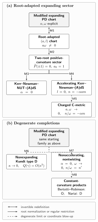
Local relations among aligned Einstein–Maxwell–$\Lambda$ solutions. Double arrows denote invertible redefinitions on their stated nondegenerate domains, solid arrows denote root normalizations or regular restrictions, and dashed arrows denote limiting procedures with held-fixed ratios or $\kappa$-dependent coordinate blow-ups. In particular, the charged C-metric retains $n/\omega=-\alpha m$. The graph makes no claim about global extensions, root cells, axes, asymptotic charges, topology, uniqueness, stability, or formation. Bertotti–Robinson is type O; Nariai with $\Lambda\ne0$ is type D.

Controlled routes through the family

Nonaccelerating Kerr–Newman–NUT–(A)dS

After root adaptation, $\alpha=0$ is a regular restriction of the transformed metric. The simultaneous coefficient relations are

$$\omega^2k=(1-l^2\Lambda)(a^2-l^2),$$ $$\epsilon=1-\left(\frac{a^2}{3}+2l^2\right)\Lambda, \qquad n=l+\frac{\Lambda}{3}(a^2-4l^2)l.$$

With $x=\cos\theta$, this is Kerr–Newman–NUT–$(A)dS$. The coefficient relations follow by specializing Eqs. (14)–(16), and the resulting metric and functions appear in Eq. (20) of Griffiths and Podolský 2006, § 4.2, printed p. 12, Open PDF. The regular restriction $l=0$ gives Kerr–Newman–$(A)dS$; adding $\Lambda=0$ gives the linked Kerr–Newman family, and then $e=g=0$ gives Kerr.

The nonrotating endpoint cannot be obtained by substituting $a=0$ into the singular affine map. Taking the finite root-adapted metric to $a=0$ instead gives

$$\epsilon=1-2\Lambda l^2, \qquad n=l-\frac43\Lambda l^3, \qquad \omega^2k=l^2(\Lambda l^2-1),$$

and

$$\begin{aligned} ds^2={}&-F_l(r) \left(dt-4l\sin^2\frac\theta2\,d\phi\right)^2 +\frac{dr^2}{F_l(r)}\\ &+(r^2+l^2)(d\theta^2+\sin^2\theta\,d\phi^2), \end{aligned}$$ $$F_l(r)=\frac{ r^2-2mr-l^2+e^2+g^2 -\Lambda\left(r^4/3+2l^2r^2-l^4\right) }{r^2+l^2}.$$

This is charged Taub–NUT–$(A)dS$. With $e=g=0$ it is a vacuum-with-$\Lambda$ Taub–NUT–$(A)dS$ solution; the linked asymptotically flat vacuum Taub–NUT spacetime is obtained after also setting $\Lambda=0$. Setting $l=0$ gives the spherical lapse

$$f(r)=1-\frac{2m}{r}+\frac{e^2+g^2}{r^2} -\frac{\Lambda r^2}{3};$$

the asymptotically flat $\Lambda=0$ member is the Reissner–Nordström solution. These nonrotating reductions are derived in Griffiths and Podolský 2006, §§ 5.3 and 8.1, printed pp. 17–20 and 26, Eqs. (30)–(31) and (53)–(55), Open PDF.

Accelerating zero-NUT branch and the C-metric endpoint

On the root-adapted branch, impose zero physical NUT parameter by setting $l=0$, not $n=0$. For $a\ne0$, use the remaining scale freedom to take

$$\omega=a, \qquad k=1,$$ $$\epsilon=1-\alpha^2(a^2+e^2+g^2)-\frac{\Lambda a^2}{3}, \qquad n=-\alpha am.$$

The angular and radial functions become

$$\begin{aligned} \widetilde P(\theta)=\sin^2\theta\Bigg[{} &1-2\alpha m\cos\theta\\ &+\left(\alpha^2(a^2+e^2+g^2) +\frac{\Lambda a^2}{3}\right)\cos^2\theta \Bigg], \end{aligned}$$ $$Q(r)= (r^2-2mr+a^2+e^2+g^2)(1-\alpha^2r^2) -\frac{\Lambda}{3}(a^2+r^2)r^2.$$

This is the accelerating Kerr–Newman–$(A)dS$ branch with no physical NUT charge. The relation $n=-\alpha am$ is the quickest proof that the canonical coefficient $n$ is not the NUT parameter. The full map is given in Griffiths and Podolský 2006, § 4.3, printed pp. 12–14, Eqs. (23)–(24), Open PDF.

The charged C-metric is the degenerate endpoint

$$a\to0, \qquad \omega=a\to0, \qquad n\to0, \qquad \frac n\omega=-\alpha m \quad\text{fixed}.$$

Writing $n'=n/\omega$ before the limit gives the full finite twist-free angular polynomial

$$P_0(p)=k+2n'p-\epsilon p^2+2\alpha mp^3 -\alpha^2(e^2+g^2)p^4.$$

On the zero-NUT branch, $k=1$, $n'=-\alpha m$, and $\epsilon=1-\alpha^2(e^2+g^2)$. The resulting finite metric is

$$ds^2=\frac{1}{(1-\alpha pr)^2} \left[ -\widetilde Q_C\,d\tau^2+ \frac{dr^2}{\widetilde Q_C} +r^2\left(\frac{dp^2}{P_C}+P_Cd\sigma^2\right) \right],$$

with

$$P_C(p)=(1-p^2) \left[1-2\alpha mp+\alpha^2(e^2+g^2)p^2\right],$$ $$\widetilde Q_C(r)= (1-\alpha^2r^2) \left(1-\frac{2m}{r}+\frac{e^2+g^2}{r^2}\right) -\frac{\Lambda r^2}{3}.$$

Naively setting $n/\omega$ to zero would delete the linear term and break the paired linear–cubic structure needed for the generic $\alpha m\ne0$ factorization. The endpoint is derived both from the rotating branch and from the twist-free chart in Griffiths and Podolský 2006, §§ 4.3.1 and 6, printed pp. 14 and 20–21, Eqs. (39)–(42), Open PDF. Its axes, conical defects, and horizon domains belong to the C-metric chapter and its charged and rotating family page.

The nonexpanding Kundt branch

The expanding canonical chart does not contain the nonexpanding solutions by ordinary parameter substitution. For $\omega\ne0$, first scale $\omega=1$ and make the singular blow-up

$$r=\gamma+\kappa q, \qquad \sigma=\frac{t}{\kappa}, \qquad \tau=\psi-\frac{\gamma^2}{\kappa}t.$$

Keep

$$Q_\alpha(\gamma)=\kappa^2\epsilon_0, \qquad Q_\alpha'(\gamma)=\kappa\epsilon_1, \qquad \epsilon_2=-\frac12Q_\alpha''(\gamma)$$

finite and choose $\gamma$ so that $\epsilon_1=0$. Explicitly,

$$\epsilon_2=-\epsilon+6\alpha n\gamma +6\alpha^2k\gamma^2+2\Lambda\gamma^2.$$

After a remaining rescaling, $\epsilon_2$ may be normalized to $+1$, $-1$, or $0$. A convenient parameter form of the finite-limit constraints is

$$\epsilon=-\epsilon_2+6\alpha n\gamma +2(3\alpha^2k+\Lambda)\gamma^2,$$ $$3m+(\epsilon_2-2\epsilon)\gamma +3\alpha n\gamma^2=0,$$ $$k+e^2+g^2-\gamma m +\frac{\epsilon+\epsilon_2}{6}\gamma^2 =\kappa^2\epsilon_0\longrightarrow0.$$

The $\kappa\to0$ metric is

$$\begin{aligned} ds^2=\frac{\gamma^2+p^2}{(1-\alpha\gamma p)^2} \Bigg[{} &-\overline Q(q)\,dt^2+\frac{dq^2}{\overline Q(q)} +\frac{dp^2}{P_\alpha(p)}\\ &+\frac{P_\alpha(p)}{(\gamma^2+p^2)^2} (d\psi+2\gamma q\,dt)^2 \Bigg], \end{aligned}$$

where $\overline Q(q)=\epsilon_0-\epsilon_2q^2$. The repeated principal congruence is now geodesic, shear-free, nonexpanding, and nontwisting, so the regular nonconformally-flat members belong to the Kundt family. The transformation, finite-limit constraints, and standard Kundt conversion are given in Griffiths and Podolský 2006, § 7, printed pp. 22–25, Eqs. (43)–(52), Open PDF.

Direct-product limits

An even more specialized blow-up starts from the finite nonaccelerating, twist-free endpoint obtained by holding $n'=n/\omega$ fixed before taking $\omega\to0$, and then setting $\alpha=0$:

$$P(p)=k+2n'p-\epsilon p^2, \qquad Q(r)=e^2+g^2-2mr+\epsilon r^2-\frac{\Lambda r^4}{3}.$$

Set

$$\begin{aligned} p&=\beta+\kappa\widetilde p, &r&=\gamma+\kappa\widetilde q,\\ \sigma&=\kappa^{-1}\widetilde\sigma, &\tau&=b^2\kappa^{-1}\widetilde\tau. \end{aligned}$$

Take $b\gamma\ne0$ so the product is nondegenerate. After dividing by the two powers of $\kappa$ supplied by the coordinate blow-up, the exact polynomial expansions are

$$\begin{aligned} \widetilde P_\kappa(\widetilde p) &=a_0+a_1\widetilde p-\epsilon\widetilde p^2,\\ \widetilde Q_\kappa(\widetilde q) &=b_0+b_1\widetilde q+B_2\widetilde q^2 -\frac{4\Lambda}{3}\gamma\kappa\widetilde q^3 -\frac{\Lambda}{3}\kappa^2\widetilde q^4, \end{aligned}$$

where the finite limiting coefficients are obtained from

$$\begin{aligned} a_0&=\kappa^{-2}(k+2\beta n'-\epsilon\beta^2), &a_1&=2\kappa^{-1}(n'-\epsilon\beta),\\ b_0&=\kappa^{-2}\left(e^2+g^2-2m\gamma+\epsilon\gamma^2 -\frac{\Lambda\gamma^4}{3}\right), &b_1&=2\kappa^{-1}\left(-m+\epsilon\gamma -\frac{2\Lambda\gamma^3}{3}\right),\\ B_2&=\epsilon-2\Lambda\gamma^2. \end{aligned}$$

Thus the two constant numerators must be $O(\kappa^2)$ and the two linear numerators must be $O(\kappa)$. On the generic centered subcase with $\epsilon\ne0$ and $B_2\ne0$, the shifts may be chosen so that

$$\frac{2\Lambda}{3}\gamma^3-\epsilon\gamma+m=0, \qquad \epsilon\beta-n'=0,$$

which sets the limiting linear terms to zero. Exceptional zero-curvature cases must instead be read from the unsimplified quadratics above; the centering equations are not universal requirements.

The limit is a direct product of two constant-curvature two-geometries,

$$ds^2=b^2\left[-Y(\widetilde q)d\widetilde\tau^2 +\frac{d\widetilde q^2}{Y(\widetilde q)}\right] +\gamma^2\left[ \frac{d\widetilde p^2}{\widetilde P(\widetilde p)} +\widetilde P(\widetilde p)d\widetilde\sigma^2 \right],$$

where $\widetilde P=\lim_{\kappa\to0}\widetilde P_\kappa$, $\widetilde Q=\lim_{\kappa\to0}\widetilde Q_\kappa$, and

$$Y(\widetilde q)=\frac{b^2}{\gamma^2} \widetilde Q(\widetilde q).$$

This makes both the limiting functions and the required scaling reproducible.

For a concrete Bertotti–Robinson path, take

$$\Lambda=g=0, \quad \epsilon=1, \quad b=\gamma=m\ne0, \quad \beta=n', \quad k=-n'^2+\kappa^2.$$

The finite-limit condition forces $e^2=m^2$. Then $\widetilde P=1-\widetilde p^2$, $Y=\widetilde q^2$, and the further substitutions $\widetilde p=\cos\theta$, $\widetilde\sigma=-\phi$, and $\widetilde q=1/R$ give

$$ds^2=\frac{L^2}{R^2}(-d\widetilde\tau^2+dR^2) +L^2(d\theta^2+\sin^2\theta\,d\phi^2), \qquad L=\lvert e\rvert.$$

For an explicit Nariai path, let $\Lambda>0$, set $L=\gamma=b=\Lambda^{-1/2}$, and take

$$e=g=n'=\beta=0, \qquad \epsilon=1, \qquad k=\kappa^2, \qquad m(\kappa)=\frac{L}{3}-\frac{\kappa^2}{2L}.$$

Then $a_0=b_0=1$, $a_1=0$, $b_1\to0$, and $B_2=-1$, so

$$\widetilde P=1-\widetilde p^2, \qquad Y=1-\widetilde q^2.$$

With $\widetilde p=\cos\theta$, $\widetilde\sigma=-\phi$, and $\widetilde q=\cos\chi$, the limit becomes

$$ds^2=L^2\left( -\sin^2\chi\,d\widetilde\tau^2+d\chi^2 +d\theta^2+\sin^2\theta\,d\phi^2 \right),$$

the static patch of $dS_2\times S^2$. The general construction and its other curvature-sign choices are derived in Griffiths and Podolský 2006, § 8.2, printed pp. 27–29, Eqs. (56)–(62), Open PDF; the two named geometries are developed on Nariai and Bertotti–Robinson Geometries.

For a product of two two-dimensional constant-curvature factors with curvatures $K_1$ and $K_2$, an adapted null tetrad has

$$\Psi_0=\Psi_1=\Psi_3=\Psi_4=0, \qquad \Psi_2=-\frac{K_1+K_2}{6}.$$

Consequently,

$$C_{\mu\nu\rho\sigma}C^{\mu\nu\rho\sigma} =\frac43(K_1+K_2)^2.$$

Bertotti–Robinson has $K_1=-K_2$ and is conformally flat, hence type O. Nariai has $K_1=K_2=\Lambda\ne0$ and remains type D. A degenerate family limit can therefore change Petrov type without making the limiting metric singular.

A reliable identification workflow

A parameter map is safest in this order:

1. choose an interval with $P>0$, choose a sign cell of $Q$, and specify the conformal boundary;
2. choose which commuting Killing combinations represent time translation and $2\pi$ rotation;
3. normalize the asymptotic or background time, when such a normalization exists;
4. compute Maxwell fluxes, twist or NUT data, and asymptotic mass and angular momentum;
5. test both axis segments for conical regularity; and
6. compare curvature and algebraic invariants before declaring two limits identical.

What the synthesis does and does not prove

The family organizes local exact solutions and their algebraic relation. A root of $Q$ is only a candidate Killing horizon until its generator and extension are checked. A zero of $P$ may be an axis, but its conical regularity depends on the one global angular period. Parameters that generate acceleration can introduce cosmic-string or strut defects. NUT identifications can introduce closed timelike curves. None of those global facts follows from type D alone.

Nor does the synthesis establish uniqueness, stability, formation, or observational relevance. Its value is controlled comparison: field equations, principal null structure, parameter maps, root domains, fluxes, invariants, and limits can all be checked within one notation.

Common pitfalls

Reading $n$ as NUT charge. On the physically zero-NUT accelerating rotating branch, $l=0$ but $n=-\alpha am$. NUT behavior is identified only after the root-adapted map and global axis analysis.

Setting a scale to zero inside an invertible map. The hatted rescaling assumes nonzero $\alpha$ and $\omega$, and the affine root map assumes nonzero $a$ and $\omega$. Their endpoints must be taken in the transformed metric with finite ratios specified.

Calling every root a horizon. A $Q$ root is a candidate Killing horizon; a $P$ root is often an axis. Generator normalization, regular coordinates, angular periodicity, and curvature decide what the boundary actually is.

Calling every product type D. Bertotti–Robinson is type O, whereas Nariai is type D. “Belongs to a type-D family by degeneration” is not the same as “has Petrov type D.”

Exercises

Determinants and sign cells

Starting from the one-forms $u$ and $v$, derive the Killing-block and full determinants. Then classify the timelike direction for $P>0$ and each sign of $Q$.

Solution

In the $(u,v)$ basis, the Killing coefficients are $\Omega^2P/\rho^2$ and $-\Omega^2Q/\rho^2$. The change from $(d\tau, d\sigma)$ has determinant $-\rho^2$, so its squared determinant contributes $\rho^4$:

$$\det g_{\rm Killing} =\rho^4\left(\frac{\Omega^2P}{\rho^2}\right) \left(-\frac{\Omega^2Q}{\rho^2}\right) =-\Omega^4PQ.$$

Multiplying by $g_{pp}=\Omega^2\rho^2/P$ and $g_{qq}=\Omega^2\rho^2/Q$ gives $\det g=-\Omega^8\rho^4$. For $P>0,Q>0$, $p$ and $q$ are spacelike and the $v$ direction is timelike. For $P>0,Q<0$, both Killing eigenvalues are positive and $g_{qq}<0$, so $q$ is timelike.

Why zero acceleration is not a direct use of the rescaling

Verify $1-\hat p\hat q=1-\alpha pr$. Why can the same formula not be used as an invertible coordinate transformation at $\alpha=0$?

Solution

The product of the transformed coordinates is

$$\hat p\hat q =\sqrt{\alpha\omega}\sqrt{\frac\alpha\omega}\,pr =\alpha pr.$$

For $\alpha>0$, the inverse transformations divide by the same nonzero scale factors. At $\alpha=0$, both $\hat p$ and $\hat q$ collapse, while the Killing-coordinate factors diverge or vanish. The Jacobian is no longer invertible. The correct nonaccelerating family is obtained by first rewriting the metric in the finite $(\alpha,\omega)$ form and only then restricting $\alpha=0$.

The zero-NUT branch and the charged C-metric

Use $l=0$, $\omega=a$, and $n=-\alpha am$ to explain why $n=0$ is not the zero-NUT condition. Then take $a\to0$ while holding $n/\omega$ fixed and recover $P_C$.

Solution

For nonzero acceleration, rotation, and mass, $l=0$ gives $n=-\alpha am\ne0$. Thus $l$, not the canonical coefficient $n$, measures physical NUT behavior on this normalized branch. Along the endpoint $\omega=a\to0$,

$$\frac n\omega=-\alpha m$$

remains finite. Substituting $k=1$, $n'=-\alpha m$, and $\epsilon=1-\alpha^2(e^2+g^2)$ into the twist-free polynomial gives

$$\begin{aligned} P_C(p) &=1-2\alpha mp -\left[1-\alpha^2(e^2+g^2)\right]p^2 +2\alpha mp^3 -\alpha^2(e^2+g^2)p^4\\ &=(1-p^2) \left[1-2\alpha mp+\alpha^2(e^2+g^2)p^2\right]. \end{aligned}$$

For $\alpha m\ne0$, setting $n'=0$ would fail this factorization and would not recover the generic charged C-metric branch. The massless or nonaccelerating subcases can legitimately have $n'=0$.

Petrov type in the product limits

For a product of two constant-curvature two-spaces, use the adapted-tetrad result

$$\Psi_0=\Psi_1=\Psi_3=\Psi_4=0, \qquad \Psi_2=-\frac{K_1+K_2}{6},$$

together with the invariant check

$$C_{\mu\nu\rho\sigma}C^{\mu\nu\rho\sigma} =\frac43(K_1+K_2)^2$$

to classify Bertotti–Robinson and Nariai.

Solution

Bertotti–Robinson has $K_1=-1/L^2$ and $K_2=+1/L^2$, so every Weyl scalar vanishes. Its regular geometry is conformally flat and therefore type O. Nariai has $K_1=K_2=\Lambda>0$, so only

$$\Psi_2=-\frac{\Lambda}{3}$$

is nonzero and the geometry is type D. As a consistency check,

$$C_{\mu\nu\rho\sigma}C^{\mu\nu\rho\sigma} =\frac{16}{3}\Lambda^2\ne0.$$

The invariant is nonzero, as required. The exercise also shows why Petrov type may change at a smooth degenerate limit; the invariant alone would not classify an arbitrary Lorentzian spacetime.

References

• Frolov, Valeri P., Pavel Krtouš, and David Kubizňák. “Black Holes, Hidden Symmetries, and Complete Integrability.” Living Reviews in Relativity 20 (2017): 6. DOI: 10.1007/s41114-017-0009-9. Open PDF.
• Griffiths, Jerry B., and Jiří Podolský. “A New Look at the Plebański–Demiański Family of Solutions.” International Journal of Modern Physics D 15, no. 3 (2006): 335–370. DOI: 10.1142/S0218271806007742. Open PDF.
• Plebański, Jerzy F., and Marek Demiański. “Rotating, Charged, and Uniformly Accelerating Mass in General Relativity.” Annals of Physics 98, no. 1 (1976): 98–127. DOI: 10.1016/0003-4916(76)90240-2.