The Reissner–Nordström Solution

Within four-dimensional, asymptotically flat, static, spherically symmetric electrovac, the construction below yields the Reissner–Nordström metric-field family. The complementary classification statement comes from the electrovac Birkhoff theorem: on its nonconstant-areal-radius branch, every local spherically symmetric electrovac solution with $\Lambda=0$ is locally of this form. The central result is

$$f(r)=1-\frac{2GM}{r} +\frac{G(Q_e^2+Q_m^2)}{r^2}.$$

The plus sign of the charge term is not inserted by analogy: it follows from the positive electromagnetic energy outside each symmetry sphere. This page derives that statement without assuming the final relation between the temporal and radial metric coefficients. It treats the local metric-field solution; roots, horizon-crossing charts, and analytic extensions belong to Reissner–Nordström horizons and extensions.

Required background. The Einstein Equation supplies the coupling of geometry to Maxwell stress–energy.

Helpful background. Deriving the Schwarzschild Metric introduces the same mass-function and time-normalization strategy. Exterior Algebra and Differential Forms supplies Hodge duals and flux integrals, while Stress–Energy and Conservation supplies the observer interpretation of $T_{\mu\nu}$; the most direct applications are electromagnetism with differential forms and electromagnetic stress–energy. The Riemann Curvature Tensor supports the Ricci checks, and Exact Solutions of Einstein’s Equations explains how to specify a spacetime and its matter fields. Causality and Global Structure and Affine and Variational Geodesics are needed only for the following horizons-and-extensions page and may be deferred.

Spherical flux before the metric is known

Use four-dimensional Einstein–Maxwell theory with $\Lambda=0$ and Gaussian electromagnetic normalization:

$$G_{\mu\nu}=8\pi G T_{\mu\nu}, \qquad dF=0, \qquad d\star F=0,$$ $$T_{\mu\nu}=\frac{1}{4\pi} \left( F_{\mu\alpha}F_\nu{}^\alpha -\frac14g_{\mu\nu}F_{\alpha\beta}F^{\alpha\beta} \right).$$

Here electrovac means that the Maxwell field is source-free and supplies the only stress–energy on the domain under study. “Source-free” means that the local current vanishes there. It does not force the flux through a sphere to vanish: a sphere surrounding the omitted region $r=0$ is not the boundary of a three-ball contained in the punctured domain. Allowing both electric and magnetic flux is called the dyonic case.

Begin on a connected asymptotically flat static interval with $r>0$ and

$$ds^2=-e^{2\Phi(r)}dt^2 +a(r)^{-1}dr^2+r^2d\Omega_2^2, \qquad a(r)>0.$$

Here $r$ is the areal radius: every symmetry sphere has geometric area $4\pi r^2$. Also $t\in\mathbb R$, $0<\theta<\pi$, and $\phi$ has period $2\pi$. The angular coordinates degenerate at the two axes, but the round spheres are smooth there. Choose $\partial_t$ future-directed at the selected asymptotic end. A convenient oriented orthonormal coframe is

$$e^{\hat0}=e^\Phi dt, \qquad e^{\hat1}=\frac{dr}{\sqrt a}, \qquad e^{\hat2}=r\,d\theta, \qquad e^{\hat3}=r\sin\theta\,d\phi.$$

Spherical symmetry permits one radial electric component and one radial magnetic component. With the site orientation,

$$F=-E(r)e^{\hat0}\wedge e^{\hat1} +B(r)e^{\hat2}\wedge e^{\hat3},$$ $$\star(e^{\hat0}\wedge e^{\hat1}) =-e^{\hat2}\wedge e^{\hat3}, \qquad \star(e^{\hat2}\wedge e^{\hat3}) =e^{\hat0}\wedge e^{\hat1}.$$

Before assigning the flux constants, write both two-forms in the coordinate basis:

$$\begin{aligned} F&=\frac{E e^\Phi}{\sqrt a}\,dr\wedge dt +Br^2\sin\theta\,d\theta\wedge d\phi,\\ \star F&=Er^2\sin\theta\,d\theta\wedge d\phi -\frac{B e^\Phi}{\sqrt a}\,dr\wedge dt. \end{aligned}$$

Taking exterior derivatives gives the entire radial Maxwell calculation:

$$\begin{aligned} dF&=(r^2B)'\,dr\wedge\sin\theta\,d\theta\wedge d\phi,\\ d\star F&=(r^2E)'\,dr\wedge\sin\theta\,d\theta\wedge d\phi. \end{aligned}$$

The factors $e^\Phi/\sqrt a$ occur only in terms proportional to $dr\wedge dt$; differentiating their radial coefficients produces $dr\wedge dr\wedge dt=0$. Thus the unknown metric functions cancel without assuming $e^{2\Phi}=a$. Maxwell’s equations now give

$$r^2E=Q_e, \qquad r^2B=Q_m,$$

Orienting each sphere by $\sin\theta\,d\theta\wedge d\phi$ identifies these constants with the geometric fluxes

$$Q_e=\frac{1}{4\pi}\int_{S_r^2}\star F, \qquad Q_m=\frac{1}{4\pi}\int_{S_r^2}F,$$

and the integrals immediately recover the signed orthonormal components

$$E(r)=\frac{Q_e}{r^2}, \qquad B(r)=\frac{Q_m}{r^2}.$$

The hats $\widehat E_r\equiv E(r)$ and $\widehat B_r\equiv B(r)$ used in the figure below emphasize that these are orthonormal radial components, not spherical-coordinate components of the two-form.

Before solving Einstein’s equation, the coordinate two-form is therefore

$$F=\frac{Q_e e^\Phi}{r^2\sqrt a}\,dr\wedge dt +Q_m\sin\theta\,d\theta\wedge d\phi.$$

The factor $e^\Phi/\sqrt a$ is essential at this stage. Replacing it by one before deriving $e^{2\Phi}=a$ would make the argument circular.

Maxwell energy, pressure, and tension

Define $Q^2\equiv Q_e^2+Q_m^2$. In the orthonormal frame the mixed stress tensor is

$$T^{\hat a}{}_{\hat b} =\rho\,\operatorname{diag}(-1,-1,1,1), \qquad \rho=\frac{Q^2}{8\pi r^4}.$$

Thus a static observer measures positive energy density $\rho$. The radial principal pressure is $p_r=-\rho$, a tension along the field lines, while the two tangential pressures are $p_\theta=p_\phi=\rho$. The trace vanishes:

$$T^{\hat a}{}_{\hat a} =-\rho-\rho+\rho+\rho=0.$$

Tracelessness will imply $R=0$, but it does not imply $R_{\mu\nu}=0$. Electromagnetism is matter even when its stress tensor has zero trace.

Integrating the radial Einstein equations

Because $r$ is itself a geometrically defined scalar, $g^{\mu\nu}\nabla_\mu r\nabla_\nu r=a(r)$ in this chart. Define the Misner–Sharp mass $m_{\rm MS}$ invariantly by

$$1-\frac{2Gm_{\rm MS}(r)}{r} \equiv g^{\mu\nu}\nabla_\mu r\nabla_\nu r =a(r),$$

and abbreviate it to $m(r)$ below. This is a geometric definition, not an arbitrary reparametrization of the radial metric coefficient.

For the unsolved metric, the two radial mixed Einstein components are

$$\begin{aligned} G^t{}_t &=\frac{ra'+a-1}{r^2} =-\frac{2Gm'}{r^2},\\ G^r{}_r &=\frac{2ra\Phi'+a-1}{r^2}. \end{aligned}$$

The $tt$ equation, $G^t{}_t=8\pi G T^t{}_t=-8\pi G\rho$, gives

$$m'(r)=4\pi r^2\rho(r) =\frac{Q^2}{2r^2}.$$

Let $M=\lim_{r\to\infty}m(r)$; at the normalized asymptotically flat end this is the ADM mass. It is independent boundary data. The charge fixes the radial variation $m'(r)$, but it does not determine $M$, which can also encode the mass associated with the omitted interior. Integration yields

$$m(r)=M-\frac{Q^2}{2r}.$$

The equality $T^t{}_t=T^r{}_r$ requires $G^t{}_t=G^r{}_r$. Subtracting the displayed components gives

$$a'=2a\Phi', \qquad e^{2\Phi}=C a.$$

Asymptotic flatness fixes $a\to1$. Rescaling the Killing time so that $g_{tt}\to-1$ fixes $C=1$. Hence $e^{2\Phi}=a\equiv f$, and the solution becomes

$$ds^2=-f(r)dt^2 +\frac{dr^2}{f(r)} +r^2d\Omega_2^2,$$ $$f(r)=1-\frac{2GM}{r} +\frac{GQ^2}{r^2}, \qquad Q^2=Q_e^2+Q_m^2,$$ $$F=\frac{Q_e}{r^2}\,dr\wedge dt +Q_m\sin\theta\,d\theta\wedge d\phi.$$

The sign of the charge term now has a transparent origin. The exact areal-radius mass balance assigns the field outside a sphere the contribution

$$M-m(r) =\int_r^\infty4\pi R^2\rho(R)\,dR =\frac{Q^2}{2r}>0.$$

Substituting the smaller interior mass $m(r)=M-Q^2/(2r)$ into $1-2Gm(r)/r$ turns the second minus sign into the positive $GQ^2/r^2$ term. This integral follows from the spherical Einstein equation; it is not a flat-space proper-volume integral on a $t=\text{constant}$ slice.

The complete chain is summarized in the figure. Follow the fluxes to their $r^{-2}$ fields, then read downward from the positive $r^{-4}$ energy density to the metric function.

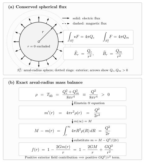
On the source-free exterior, electric and magnetic fluxes give $\widehat E_r=Q_e/r^2$ and $\widehat B_r=Q_m/r^2$. The upper panel is schematic and shows outward arrows for positive charges; reversing either charge reverses the corresponding arrows without changing the metric. The lower panel is the exact areal-radius Einstein mass balance: positive $\rho=Q^2/(8\pi r^4)$ gives $M-m(r)=Q^2/(2r)$ and therefore $f=1-2GM/r+GQ^2/r^2$. The displayed integral is not a proper-volume integral on a static slice.

Bičák displays the electric member of this family in geometrized units in Bičák 2000, §3, printed pp. 31–32, Eqs. (9)–(10), Open PDF. For that electric solution, the translation is $m_{\rm B}=GM$, $q_{\rm B}^2=GQ_e^2$, and $F_{\rm B}=\sqrt G\,F_e$ in the Gaussian normalization used here. The dyonic metric follows by the independently checked duality-invariant replacement $Q_e^2\mapsto Q_e^2+Q_m^2$; the magnetic field, flux signs, stress tensor, and radial calculation above are not claims about what is printed in that electric-only passage.

One field strength, two magnetic gauge patches

After $e^{2\Phi}=a$ is known, the final two-form can be written locally as $F=d\mathcal A$. When $Q_m\ne0$, no one smooth potential covers an entire symmetry sphere. Useful north and south potentials are

$$\begin{aligned} \mathcal A_N &=-\frac{Q_e}{r}\,dt +Q_m(1-\cos\theta)\,d\phi,\\ \mathcal A_S &=-\frac{Q_e}{r}\,dt -Q_m(1+\cos\theta)\,d\phi. \end{aligned}$$

Both give the same $F$. The first is regular at the north axis and the second at the south axis; on their overlap,

$$\mathcal A_N-\mathcal A_S=2Q_m\,d\phi.$$

The apparent axial singularity of either individual potential is a patch artifact. On the overlap the difference is locally the gauge transformation $d(2Q_m\phi)$, but $\phi$ is not a single-valued real function around the equator. The obstruction to one global smooth potential is seen directly from Stokes’ theorem: if $F=d\mathcal A$ held globally on a symmetry sphere, then

$$\int_{S^2}F =\int_{S^2}d\mathcal A =\int_{\partial S^2}\mathcal A =0,$$

contradicting $\int_{S^2}F=4\pi Q_m$ when $Q_m\ne0$. No charge quantization is assumed here; that would require additional global information about the gauge group and charged matter.

Direct checks and what the metric forgets

Substitution into the complete field equations gives

$$G^\mu{}_{\nu} =\frac{GQ^2}{r^4} \operatorname{diag}(-1,-1,1,1) =8\pi G T^\mu{}_{\nu},$$

with every off-diagonal component zero. The angular equation is therefore satisfied as well as the two radial equations. The Hodge dual of the final field is

$$\star F =Q_e\sin\theta\,d\theta\wedge d\phi -\frac{Q_m}{r^2}\,dr\wedge dt,$$

so $dF=d\star F=0$ on each displayed diagonal-chart component with $r>0$ and $f\ne0$, both flux integrals recover their defining charges, and $\star^2F=-F$. Extending that statement through a root of $f$ first requires a horizon-regular chart. The two quadratic electromagnetic invariants are

$$\begin{aligned} F_{\mu\nu}F^{\mu\nu} &=\frac{2(Q_m^2-Q_e^2)}{r^4},\\ F_{\mu\nu}(\star F)^{\mu\nu} &=\frac{4Q_eQ_m}{r^4}. \end{aligned}$$

The second sign follows from $\epsilon_{tr\theta\phi}=+\sqrt{-g}$, the site Hodge convention, and the ordering $dr\wedge dt$ in $F$.

For a constant duality angle $\beta$, define

$$F_\beta=F\cos\beta+\star F\sin\beta.$$

Since $\star^2=-1$ on two-forms, its flux charges are

$$\begin{pmatrix}Q_{e,\beta}\\ Q_{m,\beta}\end{pmatrix} = \begin{pmatrix} \cos\beta&-\sin\beta\\ \sin\beta&\cos\beta \end{pmatrix} \begin{pmatrix}Q_e\\Q_m\end{pmatrix},$$

so $Q_{e,\beta}^2+Q_{m,\beta}^2=Q^2$. For $Q>0$, writing $Q_e=Q\cos\alpha$ and $Q_m=Q\sin\alpha$ makes the action simply $\alpha\mapsto\alpha+\beta$. The neutral case $Q=0$ needs no angle. The metric and stress tensor remember only $Q^2$, whereas the ordered invariant pair changes with $2\alpha$. Even that pair determines $\alpha$ only modulo $\pi$, because $F$ and $-F$ have the same quadratic invariants. Thus two solutions can have the same metric while differing as metric-field solutions.

Tracing Einstein’s equation gives $R=0$. For $Q\ne0$, however, the displayed Einstein tensor proves that $R_{\mu\nu}\ne0$. The detailed curvature invariants and the central singularity test are developed on invariants, singularities, and controlled limits.

Domain and controlled limits

The derivation began on the asymptotically flat static component, where $f>0$ and $\partial_t$ is timelike. The final diagonal coordinates define a Lorentzian chart on any connected interval with $r>0$ and $f\ne0$; where $f<0$, $r$ is timelike and $t$ is spacelike. A zero of $f$ is excluded from this diagonal chart, not automatically from the spacetime. Its regular extension and causal meaning require the next page.

Three checks should be immediate:

Operation	Result	What it checks
$Q_e=Q_m=0$	Schwarzschild with $f=1-2GM/r$	Neutral limit and mass normalization
$M=Q_e=Q_m=0$	Minkowski metric on the $r>0$ spherical chart; its regular centre may then be adjoined	Joint flat limit and the distinction between a chart domain and the completed flat spacetime
$r\to\infty$	$g_{tt}=-1+2GM/r+O(r^{-2})$ and $F_{\hat a\hat b}=O(r^{-2})$	ADM mass and asymptotic flatness

The local solution allows real $M,Q_e,Q_m$. Black-hole parameter restrictions, root multiplicities, extremality, and the distinction between Killing, event, and Cauchy horizons are deliberately deferred to Reissner–Nordström horizons and extensions. In rationalized units, or when $G$ is absorbed into charge, the printed charge term changes; use the complete Gaussian-to-rationalized map rather than restoring one factor in isolation.

Common pitfalls

Source-free does not mean zero flux. It means $dF=d\star F=0$ on the domain. A sphere surrounding an omitted region can carry nonzero conserved flux.

The positive charge term does not represent negative field energy. The energy density is positive. The plus sign appears because the mass function inside radius $r$ is the asymptotic mass minus the positive exterior field contribution.

Zero scalar curvature does not mean vacuum or flatness. Maxwell stress is trace free, so $R=0$, but $R_{\mu\nu}$ and the full curvature remain nonzero when $Q\ne0$.

The metric does not determine the electromagnetic field. It fixes $Q_e^2+Q_m^2$, not the charge signs or electric–magnetic duality angle.

A gauge-potential singularity need not be a field singularity. For magnetic charge, north and south potentials are individually regular on their own patches and produce one smooth field strength on the sphere.

Exercises

Recover the coordinate field without circular reasoning

Starting from the orthonormal coframe and

$$F=-\frac{Q_e}{r^2}e^{\hat0}\wedge e^{\hat1} +\frac{Q_m}{r^2}e^{\hat2}\wedge e^{\hat3},$$

derive the coordinate expression before and after $e^{2\Phi}=a$ is known.

Solution

The coframe gives

$$e^{\hat0}\wedge e^{\hat1} =\frac{e^\Phi}{\sqrt a}\,dt\wedge dr, \qquad e^{\hat2}\wedge e^{\hat3} =r^2\sin\theta\,d\theta\wedge d\phi.$$

Because $dt\wedge dr=-dr\wedge dt$,

$$F=\frac{Q_e e^\Phi}{r^2\sqrt a}\,dr\wedge dt +Q_m\sin\theta\,d\theta\wedge d\phi.$$

Only after the Einstein equations and asymptotic normalization give $e^{2\Phi}=a$ does the ratio become one, producing the final coordinate field.

Derive the Maxwell principal pressures

Use the orthonormal electric and magnetic components to verify the displayed stress tensor, including its trace.

Solution

The electric and magnetic fields are parallel to the radial basis vector. In Gaussian units the energy density is

$$\rho=\frac{E^2+B^2}{8\pi} =\frac{Q_e^2+Q_m^2}{8\pi r^4}.$$

For orthonormal spatial indices, the Maxwell tensor can be written

$$T_{\hat0\hat0}=\frac{E^2+B^2}{8\pi}, \qquad T_{\hat i\hat j} =\frac{1}{8\pi} \left[(E^2+B^2)\delta_{ij} -2(E_iE_j+B_iB_j)\right].$$

Choose the first spatial basis vector to be radial. Then $E_i=(E,0,0)$ and $B_i=(B,0,0)$, so

$$T_{\hat1\hat1}=-\rho, \qquad T_{\hat2\hat2}=T_{\hat3\hat3}=\rho.$$

Raising the first index changes the sign of the time component but not the spatial components. Hence

$$T^{\hat a}{}_{\hat b} =\operatorname{diag}(-\rho,-\rho,\rho,\rho),$$

whose trace is $-\rho-\rho+\rho+\rho=0$.

Explain the sign of the charge correction

Integrate the mass equation using $m(\infty)=M$ and recover $f(r)$.

Solution

From $m'=Q^2/(2r^2)$,

$$M-m(r)=\int_r^\infty\frac{Q^2}{2R^2}\,dR =\frac{Q^2}{2r}.$$

Therefore $m=M-Q^2/(2r)$, and

$$1-\frac{2Gm}{r} =1-\frac{2GM}{r}+\frac{GQ^2}{r^2}.$$

The field energy is positive; the plus sign results from subtracting that positive exterior contribution from the asymptotic mass before inserting $m(r)$ into the metric.

Check the remaining Einstein equation

For a metric $ds^2=-fdt^2+f^{-1}dr^2+r^2d\Omega_2^2$, the mixed angular component is

$$G^\theta{}_\theta =G^\phi{}_\phi =\frac12f''+\frac{f'}{r}.$$

Substitute the Reissner–Nordström function and compare with Maxwell stress. Why is this also consistent with the Bianchi identity?

Solution

For

$$f=1-\frac{2GM}{r}+\frac{GQ^2}{r^2},$$

direct differentiation gives

$$\frac12f''+\frac{f'}r =\frac{GQ^2}{r^4} =8\pi G T^\theta{}_\theta.$$

The same holds for the $\phi$ component. More structurally, $\nabla_\mu G^\mu{}_\nu=0$ by the contracted Bianchi identity, while the source-free Maxwell equation gives $\nabla_\mu T^\mu{}_\nu=0$. Once the two independent radial Einstein equations and Maxwell’s equation hold on a regular radial interval, the conservation identity makes the angular residual dependent rather than a new integration equation. Direct substitution verifies the result without relying on that structural argument alone.

Prove why magnetic charge needs two gauge patches

Verify that the north and south potentials give the same magnetic field, find their difference on the overlap, and use Stokes’ theorem to rule out one globally smooth potential on $S^2$ when $Q_m\ne0$.

Solution

Restricting to a sphere of fixed $t$ and $r$ gives

$$d\!\left[Q_m(1-\cos\theta)d\phi\right] =Q_m\sin\theta\,d\theta\wedge d\phi,$$

and the same derivative follows from $-Q_m(1+\cos\theta)d\phi$. Their overlap difference is $2Q_m d\phi=d(2Q_m\phi)$ locally. If a single smooth potential existed on the whole sphere, however, then

$$4\pi Q_m=\int_{S^2}F=\int_{S^2}d\mathcal A =\int_{\partial S^2}\mathcal A=0,$$

which is impossible for $Q_m\ne0$. The two-patch description is therefore not optional gauge clutter; it represents the nonzero magnetic flux.

Rotate electric charge into magnetic charge

For $F_\beta=F\cos\beta+\star F\sin\beta$, derive the transformed electric and magnetic charges and show that the metric function is unchanged.

Solution

Using $\star^2F=-F$,

$$\star F_\beta=\star F\cos\beta-F\sin\beta.$$

Integrating $\star F_\beta$ and $F_\beta$ over a symmetry sphere gives

$$Q_{e,\beta}=Q_e\cos\beta-Q_m\sin\beta, \qquad Q_{m,\beta}=Q_e\sin\beta+Q_m\cos\beta.$$

This is an ordinary rotation, so $Q_{e,\beta}^2+Q_{m,\beta}^2=Q_e^2+Q_m^2$. The lapse depends on the charges only through this sum, and therefore remains unchanged. For example, a purely electric field with $Q_e=Q$, $Q_m=0$ becomes purely magnetic at $\beta=\pi/2$.

References

• Bičák, Jiří. “Selected Solutions of Einstein’s Field Equations: Their Role in General Relativity and Astrophysics.” In Einstein’s Field Equations and Their Physical Implications, edited by Bernd G. Schmidt, Lecture Notes in Physics 540, 1–126. Berlin: Springer, 2000. DOI: 10.1007/3-540-46580-4_1. Open PDF.