Light Bundles and Area Distance

A single null geodesic gives a direction but no image size. Observable angular size and geometric-optics flux require a two-parameter bundle of neighboring rays. The Jacobi map sends a small angular separation at an observer to a transverse separation along the beam; its determinant defines area distance, while its loss of rank identifies caustics. Curvature changes this map through geodesic deviation, not by changing a coordinate radius.

Required background. Classical Fields and Their Actions supplies the electromagnetic quantity transported by a bundle; The Wave Equation and Characteristics supplies the ray limit; Affine Connections and Covariant Derivatives supplies parallel transport and curvature commutators.

Helpful background. Events, Intervals, and Minkowski Geometry reviews the observer’s celestial sphere; Tensor Fields and Natural Operations reviews linear maps and determinants; Timelike Congruences and Spatial Projection prepares expansion, shear, and vorticity.

Screen Jacobi fields

Let $x^\mu(\lambda)$ be an affinely parametrized null ray with tangent $k^\mu$. Choose a parallel-transported screen basis $E_A^\mu$, $A=1,2$, satisfying

$$E_A\cdot E_B=\delta_{AB}, \qquad E_A\cdot k=0, \qquad k^\nu\nabla_\nu E_A^\mu=0.$$

A connecting field $\xi^\mu$ to a neighboring ray obeys the Jacobi equation in the site curvature convention,

$$\frac{D^2\xi^\mu}{d\lambda^2} =R^\mu{}_{\nu\rho\sigma} k^\nu k^\rho\xi^\sigma.$$

Longitudinal multiples of $k^\mu$ merely relabel points along a generator. The physical transverse part can be written

$$\xi_\perp^\mu =E_A^\mu\mathcal D^A{}_B(\lambda)\alpha^B,$$

where $\alpha^B$ is a small angular vector at the observer. The Jacobi matrix satisfies

$$\frac{d^2\mathcal D^A{}_B}{d\lambda^2} =\mathcal R^A{}_C\mathcal D^C{}_B,$$

with $\mathcal R$ the screen projection of the curvature operator $\xi^\mu\mapsto R^\mu{}_{\nu\rho\sigma}k^\nu k^\rho\xi^\sigma$. This second-order formulation remains regular when the first-order optical scalars diverge. Perlick 2010, §2.3, pp. 13–17, PDF gives the Jacobi-matrix and Sachs descriptions side by side, with its curvature signs fixed by its stated convention.

Vertex data and area distance

Place the bundle vertex at the observation event $O$, set $\lambda(O)=0$, and normalize

$$-u_O\cdot k_O=1.$$

Then an angular perturbation has the canonical initial data

$$\mathcal D(0)=0, \qquad \mathcal D'(0)=I.$$

This normalization takes $k$ future directed. For a source on the observer’s past light cone, follow the same geodesic backward to $\lambda\lt0$; $\alpha^A$ uses the corresponding orientation of the screen basis. Equivalently one may use a past-directed tangent and a positive parameter into the past, changing both the tangent normalization and initial-data signs consistently. The absolute determinant makes the area distance independent of this orientation choice.

For an infinitesimal solid angle $d\Omega_O$, the beam’s cross-sectional area at $\lambda$ is

$$d\mathscr S(\lambda) =\left|\det\mathcal D(\lambda)\right|d\Omega_O.$$

The angular-diameter, or area, distance is therefore

$$D_A^2=\left|\det\mathcal D\right|.$$

It depends on the observer velocity through the normalization and observed solid angle. It is not generally a coordinate separation, and it need not grow monotonically. The precise operational definition, extremal angular distances, parity, and observer dependence are detailed in Perlick 2010, §2.4, pp. 19–21, PDF.

On any interval where $\mathcal D$ is invertible, define $\mathcal B=\mathcal D'\mathcal D^{-1}$. Then

$$\Theta=\operatorname{tr}\mathcal B =\frac{d}{d\lambda}\ln|\det\mathcal D|, \qquad \frac{D_A'}{D_A}=\frac12\Theta.$$

For a wavefront bundle the twist vanishes. If $\sigma^2\equiv\tfrac12\sigma_{AB}\sigma^{AB}$, null Raychaudhuri evolution gives the area focusing equation

$$D_A'' =-\left( \frac12R_{\mu\nu}k^\mu k^\nu+\sigma^2 \right)D_A$$

between caustics. To see the factors, differentiate $\mathcal B=\mathcal D'\mathcal D^{-1}$ to get $\mathcal B'=\mathcal R-\mathcal B^2$. The screen curvature has trace $\operatorname{tr}\mathcal R=-R_{\mu\nu}k^\mu k^\nu$. For vanishing twist, $\mathcal B=\tfrac12\Theta I+\sigma$, so $\Theta'=-R_{\mu\nu}k^\mu k^\nu-\tfrac12\Theta^2-2\sigma^2$. Combining this with $D_A'/D_A=\Theta/2$ gives the displayed focusing equation. Ricci curvature supplies the isotropic term, whose sign focuses only when $R_{\mu\nu}k^\mu k^\nu\ge0$; Weyl curvature generates shear and thereby also changes the area.

Caustics, parity, and magnification

A caustic or conjugate point occurs when $\det\mathcal D=0$. Rank one means collapse in one transverse direction; rank zero means both directions collapse. The matrix $\mathcal D$ itself can remain smooth through the event, but $\mathcal B$ and the geometric-optics amplitude generally diverge because they require $\mathcal D^{-1}$ or $D_A^{-1}$; Dolan 2018, §§4.1–4.2, pp. 9–11, PDF exhibits this contrast between regular deviation fields and singular optical scalars. A signed determinant records image parity across the caustic; the nonnegative $D_A$ deliberately discards that sign.

The figure makes the rank change geometrically visible. Inspect how the two singular values $s_1,s_2$ of the screen map become the ellipse semiaxes, so $D_A^2=s_1s_2=|\det\mathcal D|$, and how losing only the smaller one is already enough to destroy the inverse. The figure writes $D$ for the same Jacobi map denoted $\mathcal D$ on this page, and its overdot is this page’s prime: both mean $d/d\lambda$.

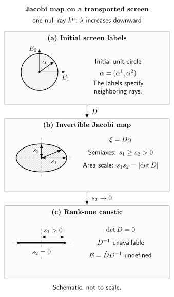
The Jacobi map carries initial transverse labels to screen separations. Before the caustic its singular values are the beam ellipse semiaxes and B=dot D D^-1; when one stretch vanishes, D loses rank and the inverse-based optical tensor fails although the Jacobi equation may remain regular. Schematic and not to scale.

Magnification is a comparison, not an absolute local scalar. Given a specified reference Jacobi map with the same endpoint and observer normalization, a signed area magnification is proportional to

$$\mu=\frac{\det\mathcal D_{\rm ref}}{\det\mathcal D}.$$

Without the reference model and endpoint prescription, calling a beam “magnified” is incomplete. Detailed observational lens models, finite sources, and image reconstruction lie outside this page.

Approximation boundary and checks

The bundle construction assumes vacuum geometric optics with $\varepsilon=\lambda_{\rm red}/L\ll1$ and infinitesimal angular width. It retains the leading ray and Jacobi equations while discarding finite-frequency phase and diffraction corrections, normally relative $O(\varepsilon)$ away from singular regions. Near a caustic the remainder is not uniform: wave interference smooths the ray-optics divergence over a scale set by wavelength. A dispersive medium replaces the metric Jacobi problem by deviation for a frequency-dependent Hamiltonian flow, so the distance can depend on frequency and polarization.

As an independent local check, regular curvature and the vertex data imply

$$\mathcal D(\lambda)=\lambda I+O(\lambda^3), \qquad D_A=|\lambda|+O(\lambda^3).$$

The absence of a quadratic term follows directly from $\mathcal D''(0)=\mathcal R(0)\mathcal D(0)=0$. It recovers the locally Minkowskian solid-angle law.

Exercise

Solve the Jacobi-map problem for a vertex bundle in Minkowski spacetime and connect it to amplitude transport.

Solution

Flat spacetime has $\mathcal R=0$, so

$$\mathcal D''=0, \qquad \mathcal D(0)=0, \qquad \mathcal D'(0)=I$$

gives $\mathcal D=\lambda I$. Hence

$$D_A=|\lambda|, \qquad \Theta=\frac2\lambda.$$

The beam area is proportional to $\lambda^2$. Since $\mathcal A^2\mathscr S$ is conserved, $\mathcal A\propto|\lambda|^{-1}$, reproducing the radial flat-space result without referring to a coordinate radius.

References

• Dolan, Sam R. “Geometrical Optics for Scalar, Electromagnetic and Gravitational Waves on Curved Spacetime.” International Journal of Modern Physics D 27 (2018): 1843010. DOI. Open PDF.
• Perlick, Volker. “Gravitational Lensing from a Spacetime Perspective.” Living Reviews in Relativity 7 (2004): 9; revised arXiv version, 2010. DOI. Open PDF.