Observer Tidal Tensors

A local array of freely falling probes does not read an arbitrary coordinate component of curvature. It reads the electric Riemann tensor selected by the array’s reference observer. This tensor is a symmetric spatial $3\times3$ map with six independent components, completely determined by the instantaneous relative accelerations of three linearly independent, initially comoving separations. Its trace and its distinction from electric Weyl curvature identify what matter-associated information is present.

Required background. Affine and Variational Geodesics supplies the Jacobi field; The Riemann Curvature Tensor supplies the Riemann symmetries and Weyl decomposition; Observers, Rest Spaces, and Measured Components supplies rest-space projections and tetrads.

Helpful background. Events, Intervals, and Minkowski Geometry reviews orthonormal frames; Tensor Fields and Natural Operations reviews contractions and basis changes; The Newtonian Gravitational Field and Potential supplies the Hessian interpretation.

The electric Riemann tensor of an observer

Let $u^\mu$ be a unit future-directed four-velocity and

$$h_{\mu\nu}=g_{\mu\nu}+u_\mu u_\nu$$

its rest-space metric. Define the observer’s electric Riemann tensor by

$$\mathcal E_{\mu\nu}(u) \equiv R_{\mu\alpha\nu\beta}u^\alpha u^\beta.$$

The Riemann antisymmetries imply $\mathcal E_{\mu\nu}u^\nu=0$, and pair exchange implies $\mathcal E_{\mu\nu}=\mathcal E_{\nu\mu}$. In an orthonormal tetrad $e_{\hat0}=u$, only $\mathcal E_{\hat i\hat j}=R_{\hat i\hat0\hat j\hat0}$ remain. A symmetric three-dimensional tensor has six independent components. These are statements about a specified observer; changing $u$ changes the contraction, not merely the displayed basis.

The underlying geodesic-deviation construction and its operational interpretation are established in Reall 2013, §6.5, pp. 60–62, PDF and Carroll 1997, §3, pp. 85–88, PDF.

Reading the six components with a probe array

Choose a parallel-propagated tetrad on a reference geodesic. At one event, release three nearby probes with independent spatial separations $\xi_{(A)}^{\hat i}$ and zero relative velocity in that tetrad. To first order,

$$a_{(A)}^{\hat i} \equiv\frac{d^2\xi_{(A)}^{\hat i}}{d\tau^2} =-\mathcal E^{\hat i}{}_{\hat j}\xi_{(A)}^{\hat j}.$$

Assemble the separations and accelerations as matrices $X^{\hat i}{}_A$ and $A^{\hat i}{}_A$. If $X$ is invertible,

$$\mathcal E=-AX^{-1}.$$

For separations aligned with an orthonormal triad and all having length $L$, the $A$th acceleration vector gives the negative of the $A$th column of $L\mathcal E$. Equality of the inferred off-diagonal entries is an internal symmetry check. Diagonalizing $\mathcal E$ identifies three principal tidal directions; a positive eigenvalue means compression in the relative-acceleration map $-\mathcal E$, while a negative eigenvalue means stretching.

The apparatus must be infinitesimal relative to curvature-variation scales, the probes must be test bodies, and accelerations must be compared at a shared proper-time convention. A Jacobi field can have an infinitesimal initial relative velocity without altering the displayed covariant equation. A relative velocity that stays finite as the baseline shrinks, finite-separation corrections, rotation of the tetrad, and nongravitational forces require additional terms. Choosing initially comoving probes makes the instantaneous measurement and its interpretation especially direct.

Ricci trace and Weyl tides

The electric Riemann tensor is not generally trace-free:

$$\mathcal E^\mu{}_\mu =R_{\alpha\beta}u^\alpha u^\beta.$$

Thus its isotropic trace samples Ricci curvature along the observer. Only after imposing a gravitational field equation may that contraction be interpreted in terms of matter variables. The trace-free part also contains freely propagating or externally sourced tidal information.

In four dimensions it is useful to define the electric and magnetic Weyl tensors,

$$E^{(C)}_{\mu\nu}=C_{\mu\alpha\nu\beta}u^\alpha u^\beta, \qquad B^{(C)}_{\mu\nu}=({}^\star C)_{\mu\alpha\nu\beta}u^\alpha u^\beta,$$

where the left dual is $({}^\star C)_{\mu\alpha\nu\beta}=\tfrac12\epsilon_{\mu\alpha}{}^{\rho\sigma}C_{\rho\sigma\nu\beta}$. Both are spatial, symmetric, and trace-free, so each has five independent components. The trace-free Weyl algebra and orthonormal-tetrad machinery used in this observer decomposition are reviewed in Carroll 1997, §3, pp. 82–92, PDF.

An initially comoving, nonrotating array directly measures the full electric Riemann tensor $\mathcal E$, not $B^{(C)}$ separately. Magnetic curvature influences velocity-dependent relative motion, precession, and holonomy. Likewise, spatial-spatial Riemann components do not appear in the single array’s instantaneous Jacobi equation. Rotating the same array within its rest space only changes the matrix representation of the same six-component tensor.

Independent algebraic checks

Spatiality follows immediately because contracting either free slot of $\mathcal E_{\mu\nu}$ with $u$ places a symmetric product $u^\mu u^\alpha$ against an antisymmetric Riemann pair. Symmetry follows from $R_{\mu\alpha\nu\beta}=R_{\nu\beta\mu\alpha}$. These two checks reduce the apparent ten components of a symmetric spacetime tensor to six rest-space components.

In the Newtonian regime, $\mathcal E_{ij}=\partial_i\partial_j\Phi$. The trace then gives $4\pi G\rho$, and the vacuum point-mass eigenvalues $(-2,1,1)GM/r^3$ reproduce radial stretching and transverse compression through $-\mathcal E$. This simultaneously checks normalization, sign, and the interpretation of the trace.

To see the deformation rather than only its signs, set $\kappa=GM/r^3$ at the reference event. If the probes are initially comoving and their radial and transverse separations both have magnitude $L$, Taylor expansion of $\ddot{\boldsymbol\xi}=-\mathcal E\boldsymbol\xi$ gives

$$\xi_{\hat r}(\Delta\tau) =L\left(1+\kappa\Delta\tau^2\right)+O(\Delta\tau^3), \qquad \xi_{\hat\perp}(\Delta\tau) =L\left(1-\frac12\kappa\Delta\tau^2\right)+O(\Delta\tau^3).$$

Thus the two transverse directions respond equally, whereas the radial coefficient is twice as large and has the opposite sign. The figure shows one radial–transverse cross-section; inspect the arrow directions before comparing them with the short-time ellipse.

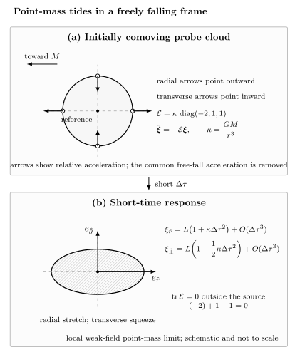
In the weak vacuum field of a point mass, $\mathcal E_{\hat i\hat j}=(GM/r^3)\operatorname{diag}(-2,1,1)$, so $-\mathcal E$ stretches an initially comoving spherical probe cloud radially and compresses both transverse directions. The zero trace reflects $R_{\mu\nu}u^\mu u^\nu=0$ outside the source. The lower panel is an $e_{\hat r}$–$e_{\hat\theta}$ cross-section; the omitted $e_{\hat\phi}$ semiaxis has the same transverse compression. Schematic and not to scale; arrows show relative rather than common free-fall acceleration.

Exercises

1. Count the readings. Why do three independent separation vectors suffice to determine $\mathcal E_{\hat i\hat j}$?

Solution

Each separation supplies a three-component acceleration, so an invertible $X$ gives all nine entries of $-AX^{-1}$. Curvature predicts that this matrix is symmetric; the three antisymmetric combinations are consistency checks, leaving the expected six independent values.

2. Isotropic curvature. If $\mathcal E_{\hat i\hat j}=K\delta_{ij}$, how does a small spherical cloud initially at rest respond?

Solution

Every separation obeys $\ddot{\boldsymbol\xi}=-K\boldsymbol\xi$. For $K>0$ the cloud initially contracts isotropically; for $K<0$ it expands isotropically. Its trace is $3K=R_{\mu\nu}u^\mu u^\nu$, so this is not a vacuum electric Riemann tensor unless $K=0$.

3. Diagnose a false reconstruction. An experimenter rotates one array through many spatial orientations and claims to have measured all twenty Riemann components. What is missing?

Solution

Every rotation preserves the same four-velocity $u$ and merely transforms $\mathcal E\mapsto Q\mathcal E Q^{\mathsf T}$. The data still contain only six independent components. Boosted observers or measurements sensitive to other curvature bivectors, such as loop holonomy or gyroscope transport, are needed to access the mixed and spatial sectors.

References

• Carroll, Sean M. “Lecture Notes on General Relativity.” arXiv:gr-qc/9712019 (1997), §3, pp. 82–92. PDF.
• Reall, Harvey S. General Relativity. Cambridge Part III lecture notes, 2013, §6.5, pp. 60–62. PDF.