Electromagnetism with Differential Forms

Differential forms compress Maxwell theory into two equations while revealing which structures do the work. The exterior derivative encodes local closure and conservation; the Hodge star introduces the metric and orientation; Stokes’ theorem produces integral flux laws; cohomology decides whether a potential can be chosen globally.

Required background. Special Relativity supplies the Minkowski metric, Lorentz covariance, and index operations; Calculus and Linear Algebra supplies multivariable differentiation and integration; Differential Forms and Integration supplies wedge products, exterior derivatives, pullbacks, orientation, and Stokes’ theorem. Helpful background. Ordinary Differential Equations supplies initial-value reasoning.

The forms and their degrees

In positively oriented inertial Cartesian coordinates, $\epsilon_{0123}=+1$; in general coordinates the inherited convention is $\epsilon_{0123}=+\sqrt{-g}$. For a $p$-form $\omega$, define

$$(\star\omega)_{\mu_{p+1}\ldots\mu_4} =\frac{1}{p!}\, \omega^{\mu_1\ldots\mu_p} \epsilon_{\mu_1\ldots\mu_4}.$$

In four-dimensional Lorentzian spacetime,

$$\star\star\omega=(-1)^{1+p(4-p)}\omega,$$

so $\star\star F=-F$ for a two-form. The objects in Maxwell theory have the following degrees:

Object	Degree	Meaning
$A$	1	Local gauge potential
$j=J_\mu dx^\mu$	1	Metric-lowered electric current
$F=dA$	2	Electromagnetic field strength
$\star F$	2	Metric-dual field strength
$\mathcal J=\star j$	3	Electric current form integrated over three-surfaces
$dF$, $d\star F$	3	Maxwell equations
$d\mathcal J$	4	Local charge conservation

The diagram traces these dependencies. Follow the solid arrows to see what the exterior derivative does without a metric; the dashed arrows mark the two places where the Hodge star needs the metric and orientation.

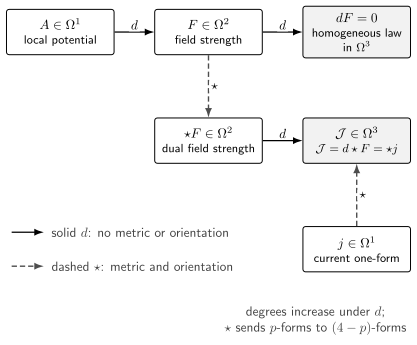
Exterior differentiation raises degree without using the metric: locally $A$ maps to $F$, and $d$ maps $F$ to the three-form $dF$, which the homogeneous equation sets to zero; separately, $d\star F$ equals the source three-form $\mathcal J$. Among the displayed operations, the dashed Hodge-star arrows are where the metric and orientation enter. Schematic dependency diagram.

On a constant-time spatial slice, let $\star_3$ be the Euclidean spatial Hodge star and let $\flat$ lower spatial vector indices. Then

$$\begin{aligned} F&=-dt\wedge E^\flat+\star_3B^\flat,\\ \star F&=dt\wedge B^\flat+\star_3E^\flat,\\ j&=-\rho\,dt+J^\flat,\\ \mathcal J=\star j&=\rho\,\mathrm{vol}_3 -dt\wedge\star_3J^\flat. \end{aligned}$$

Thus $F_{0i}=-E_i$, $F_{ij}=\epsilon_{ijk}B^k$, $(\star F)_{0i}=B_i$, and $(\star F)_{ij}=\epsilon_{ijk}E^k$. These component identities provide a direct sign check on the abstract formulas.

Maxwell’s equations and geometric dependence

The complete equations are

$$\boxed{dF=0,} \qquad \boxed{d\star F=\mathcal J=\star j.}$$

With the conventions above, the second equation is equivalent to

$$\partial_\mu F^{\mu\nu}=-J^\nu.$$

Carroll 1997, Chapter 1, printed pp. 20–24, PDF develops the field tensor, exterior derivative, Lorentzian Hodge star, and form equations. Carroll uses Gaussian normalization and a different antisymmetric index order; removing the factor $4\pi$ and translating the full convention set gives the equations displayed here. Guth 2018, Problem 1(a)–(e), pp. 1–2, PDF supplies an independent check in the same metric signature, including $\star\star F=-F$.

The two equations have different geometric content:

• $dF=0$ uses the differentiable structure but no metric. Wherever one potential exists, it is the identity $dF=d^2A=0$.
• $d\star F=\mathcal J$ uses the metric and orientation through $\star$. It is the sourced dynamical equation.
• Integrating either equation requires oriented chains and pullbacks, but no coordinate decomposition.
• Deciding whether a closed form is globally exact depends on topology.

Applying $d$ to the sourced equation gives

$$0=d^2\star F=d\mathcal J.$$

This is charge conservation. In form language, conservation is the integrability condition that a source must satisfy before $d\star F=\mathcal J$ can have a solution.

Stokes’ theorem and flux laws

Let $V$ be an oriented smooth three-chain contained in the physical domain. Stokes’ theorem gives

$$\int_{\partial V}F=\int_VdF=0, \qquad \int_{\partial V}\star F =\int_V\mathcal J.$$

When $V$ lies in a constant-time slice, the pullback of $F$ is $\star_3B^\flat$, the pullback of $\star F$ is $\star_3E^\flat$, and the pullback of $\mathcal J$ is $\rho\,\mathrm{vol}_3$. The two equations are therefore magnetic Gauss law and electric Gauss law in integral form.

The qualification “contained in the physical domain” is essential. If a closed surface bounds a three-chain entirely inside a source-free domain, its magnetic flux vanishes. A punctured domain can contain a closed surface that does not bound any three-chain there. Nonzero flux through such a surface does not violate Stokes’ theorem; it diagnoses the missing region or a nontrivial cohomology class.

The vector-calculus translation is developed in Guillemin and Haine 2019, §2.7, printed pp. 68–72, Open PDF, and the required manifold version of Stokes’ theorem appears in §4.6, printed pp. 147–150, Open PDF.

Local potentials and global topology

The Poincaré lemma says that every closed positive-degree form is exact on a contractible neighborhood. Hence $dF=0$ implies locally

$$F=dA.$$

Globally, a single smooth potential exists only if the de Rham cohomology class $[F]\in H^2(M)$ vanishes. Closed forms modulo exact forms define this obstruction. See Guillemin and Haine 2019, §2.6, printed pp. 64–65, and §5.1, pp. 171–172, Open PDF.

Local potentials $A_a$ on overlapping contractible patches obey

$$A_a-A_b=d\chi_{ab}$$

on each contractible overlap. On a noncontractible overlap, it can be misleading to write one globally single-valued real $\chi_{ab}$. For compact $U(1)$, the globally meaningful object is the transition function $e^{iq\chi_{ab}}$, as explained on Potentials, Gauge Freedom, and Constraints.

The dual statement also has a local/global distinction. In a source-free contractible patch, $d\star F=0$ permits a local dual potential $\star F=dC$. A global $C$ requires the corresponding cohomology class to vanish. Standard Riemannian Hodge-decomposition theorems additionally assume a suitable geometry and boundary conditions; they should not be transferred unchanged to noncompact Lorentzian spacetime.

Common pitfalls

Thinking that topology invalidates Stokes’ theorem. Stokes’ theorem applies to an actual chain in the domain. Topology changes which closed surfaces are boundaries of such chains.

Forgetting that the Hodge star is metric-dependent. The equation $dF=0$ survives a metric change as an identity. The equation $d\star F=\mathcal J$ changes because $\star$ changes.

Promoting a local potential to a global one. Closed implies locally exact, not globally exact. Check the cohomology class or all periods over closed cycles.

Exercises

A closed field with no global potential

On $\mathbb R^3\setminus\{0\}$, consider

$$F=g\sin\theta\,d\theta\wedge d\phi.$$

Show that this is a smooth closed form on the punctured domain and decide whether $F=dA$ for one smooth global one-form $A$ when $g\ne0$.

Solution

Although spherical coordinates are singular on an axis, the form itself is smooth away from the origin because

$$F=\frac{g}{r^3} \left( x\,dy\wedge dz+y\,dz\wedge dx+z\,dx\wedge dy \right).$$

Direct differentiation gives $dF=0$. On any sphere surrounding the omitted origin,

$$\int_{S^2}F =g\int_0^\pi\sin\theta\,d\theta \int_0^{2\pi}d\phi =4\pi g.$$

If a global smooth $A$ existed, Stokes’ theorem on the closed two-manifold $S^2$ would give $\int_{S^2}dA=\int_{\partial S^2}A=0$, contradicting the nonzero period. Local northern and southern potentials can be used instead. On a good cover their differences are exact on contractible overlaps; in a compact $U(1)$ description, the transition functions must be single-valued. With charged matter this gives the integrality condition

$$q\int_{S^2}F\in2\pi\mathbb Z.$$

The patch construction and its single-valuedness condition are developed in Tong 2018, §1.1.2, printed pp. 6–8, PDF.

Charge balance through a spacetime slab

Let $W=[t_1,t_2]\times V$ for a fixed spatial volume $V$. Integrate $d\mathcal J=0$ over $W$ and interpret the result.

Solution

Stokes’ theorem gives $\int_{\partial W}\mathcal J=0$. The final slice has positive orientation, the initial slice negative orientation, and the timelike wall records outward current. Therefore

$$Q(t_2)-Q(t_1) +\int_{t_1}^{t_2}dt \int_{\partial V}\mathbf J\mathbin{\cdot}\mathbf n\,dA=0,$$

where $Q(t)=\int_V\rho\,d^3x$. Charge can change inside $V$ only by flux through its boundary. This is the integral continuity equation with all orientation signs fixed by the boundary orientation of $W$.

Next, Electromagnetic Invariants and Field Classification uses $F$ and $\star F$ to decide which electric–magnetic mixtures a Lorentz boost can simplify.

References

• Sean M. Carroll, “Lecture Notes on General Relativity”, Chapter 1, printed pp. 20–24, arXiv:gr-qc/9712019, 1997.
• Victor Guillemin and Peter J. Haine, Differential Forms, World Scientific, 2019, ISBN 978-981-3272-77-4, DOI 10.1142/11058, Open PDF.
• Alan H. Guth, Physics 8.962: General Relativity, Problem Set 12 (PDF), Problem 1(a)–(e), pp. 1–2, Massachusetts Institute of Technology, May 5, 2018.
• David Tong, Gauge Theory (PDF), §1.1.2, printed pp. 6–8, University of Cambridge lecture notes, 2018.