Perturbation Theory, Adiabatic Evolution, and WKB

Weak static coupling, weak accumulated transitions, slow gapped driving, and short spatial wavelength are four different approximation limits. Their dimensionless controls answer different questions, and each fails at a different boundary. This page derives all four diagnostics, checks them against exact two-level and barrier results, and keeps their errors separate.

Required background. Calculus and Linear Algebra supplies eigenspaces, projections, norms, and series; Ordinary Differential Equations supplies asymptotic expansions and residual checks; Quantum States, Observables, and Measurement supplies state vectors, observables, self-adjoint operators, and domains. Helpful background. Waves, Green Functions, and Geometric Optics supplies local wavelength, eikonal, and turning-point intuition.

Quantum approximation schemes and their controls

We keep $\hbar$ explicit. The following diagnostics are local or finite-time controls, not universal convergence theorems:

Here $\lambda\in\mathbb R$ is a dimensionless bookkeeping coupling; $m,n$ label unperturbed or instantaneous eigenstates; $V_{mn}$ is a matrix element; $V_I$ is the interaction-picture perturbation; $s$ is a dimensionless slow parameter with time scale $\tau$; and $p(x)$ is the local classical momentum.

Method	Representative dimensionless control	What is assumed small	Characteristic failure
Stationary perturbation	$\lvert\lambda V_{mn}/(E_n^{(0)}-E_m^{(0)})\rvert$	Static spectral mixing	Degeneracy, small denominators, uncontrolled sums
Time-dependent perturbation	$\eta_{\rm TD}(t)=\lvert\lambda\rvert\hbar^{-1}\int_{t_0}^{t}\lVert V_I(t')\rVert dt'$	Accumulated interaction-picture action	Long duration or resonance
Adiabatic evolution	$\epsilon_{mn}^{\rm ad}=\max_s\hbar\lvert\langle m\lvert\partial_sH\rvert n\rangle\rvert/(\tau\lvert E_m-E_n\rvert^2)$	Transitions out of a slowly transported spectral band	Closing gap or insufficient regularity
WKB	$\hbar\lvert p'\rvert/\lvert p\rvert^2$	Variation of local wavelength	Turning point, discontinuity, caustic, or Stokes switching

The value of a dimensionful coupling, time, gap, or wavelength cannot by itself certify an approximation. It must appear in a dimensionless ratio or error bound.

Stationary perturbation compares mixing with gaps

To expose the spectral issue without hiding domain assumptions, first work in a finite-dimensional Hilbert space. Let $\lambda\in\mathbb R$, take $H_0=H_0^\dagger$ and $V=V^\dagger$, and choose normalized orthogonal eigenstates $|n\rangle$ of $H_0$:

$$H=H_0+\lambda V, \qquad H_0|n\rangle=E_n^{(0)}|n\rangle, \qquad V_{mn}=\langle m|V|n\rangle,$$

and suppose $E_n^{(0)}$ is isolated and nondegenerate. To second order in $\lambda$,

$$E_n=E_n^{(0)}+\lambda V_{nn} +\lambda^2\sum_{m\ne n} \frac{|V_{mn}|^2}{E_n^{(0)}-E_m^{(0)}}+O(\lambda^3),$$

while a first-order eigenvector with intermediate normalization is

$$|n\rangle_\lambda =|n\rangle+\lambda\sum_{m\ne n} \frac{V_{mn}}{E_n^{(0)}-E_m^{(0)}}|m\rangle+O(\lambda^2).$$

Here intermediate normalization means $\langle n|n\rangle_\lambda=1$ order by order; it does not impose unit norm beyond first order. In an infinite-dimensional problem these formal formulas also require control of domains, relative boundedness, and the indicated sums.

The pairwise ratios

$$\epsilon_{mn}^{\rm stat} =\left\lvert \frac{\lambda V_{mn}}{E_n^{(0)}-E_m^{(0)}} \right\rvert$$

must be small, but pairwise smallness alone need not control an infinite sum or prove convergence. For an exactly degenerate eigenspace, diagonalize the projected perturbation. For a cluster of nearly degenerate levels, let $P$ be the orthogonal projector onto that cluster and diagonalize the projected full or effective Hamiltonian $P(H_0+\lambda V)P$, including higher-order corrections induced through states outside $P$ when their size competes with the small internal gaps.

Exact two-level check

Take $\Delta\gt0$ and

$$H= \begin{pmatrix} 0&\lambda v\\ \lambda v^*&\Delta \end{pmatrix}.$$

The lower exact eigenvalue is

$$\begin{aligned} E_-&=\frac{\Delta-\sqrt{\Delta^2+4\lambda^2|v|^2}}{2}\\ &=-\frac{\lambda^2|v|^2}{\Delta} +O\!\left(\frac{\lambda^4|v|^4}{\Delta^3}\right). \end{aligned}$$

The expansion is controlled by $\epsilon_{\rm stat}=|\lambda v|/\Delta$. Its first-order energy shift vanishes, and the second-order shift has the correct negative sign for mixing with a higher level. As $\Delta\to0$, the perturbative ratio diverges while exact diagonalization gives $E_\pm=\pm|\lambda v|$.

Time-dependent perturbation controls accumulated transitions

The unitary-dynamics page derives the general change of picture. Here let $H_0$ be time independent, $H(t)=H_0+\lambda V(t)$, and $t\ge t_0$. If $U$ is the full propagator, define

$$U_0(t,t_0)=e^{-iH_0(t-t_0)/\hbar}, \qquad U_I(t,t_0)=U_0^\dagger(t,t_0)U(t,t_0),$$

and

$$V_I(t)=U_0^\dagger(t,t_0)V(t)U_0(t,t_0).$$

Then $U_I(t_0,t_0)=I$ and

$$i\hbar\,\partial_tU_I(t,t_0) =\lambda V_I(t)U_I(t,t_0).$$

Starting in the $H_0$ eigenstate $|n\rangle$, the first-order amplitude for $m\ne n$, with $V_{mn}(t)=\langle m|V(t)|n\rangle$, is

$$c_{m\leftarrow n}^{(1)}(t) =-\frac{i\lambda}{\hbar} \int_{t_0}^{t}dt'\, e^{i\omega_{mn}(t'-t_0)}V_{mn}(t'), \qquad \omega_{mn}=\frac{E_m^{(0)}-E_n^{(0)}}{\hbar}.$$

For bounded $V_I$, with $\lVert\cdot\rVert$ denoting the operator norm, a conservative sufficient finite-time control is

$$\eta_{\rm TD}(t) =\frac{|\lambda|}{\hbar} \int_{t_0}^{t}\lVert V_I(t')\rVert\,dt'\ll1.$$

The Dyson remainder after the first-order term is bounded by $e^{\eta_{\rm TD}}-1-\eta_{\rm TD}$. This norm bound ignores oscillatory cancellation and can be much stronger than necessary, but it makes one danger explicit: a weak interaction can accumulate for a long time.

For example, let $\omega\gt0$ and $V_{mn}(t)=v\cos[\omega(t-t_0)]$. Writing the cosine as two exponentials produces phases at $\omega_{mn}+\omega$ and $\omega_{mn}-\omega$. Near $\omega=|\omega_{mn}|$, one of these phases varies slowly. Over a duration $T$, suppose both

$$\bigl|\omega-|\omega_{mn}|\bigr|T\ll1, \qquad (\omega+|\omega_{mn}|)T\gg1.$$

The first condition keeps the resonant term coherent; the second makes the counter-rotating term small compared with the resonant contribution. Then, while first order remains valid,

$$\left|c_{m\leftarrow n}^{(1)}\right| \simeq\frac{|\lambda v|T}{2\hbar}.$$

Weakness at one instant does not prevent resonant growth. Near resonance, the displayed first-order result is self-consistent only while $|\lambda v|T/(2\hbar)\ll1$; an order-one amplitude calls for resummation or the exact driven two-level dynamics. At very short times with $(\omega+|\omega_{mn}|)T\ll1$, both phases are nearly constant instead, so $|c_{m\leftarrow n}^{(1)}|\simeq|\lambda v|T/\hbar$: the resonant factor of one-half must not be used before the counter-rotating term averages out. Turner derives the interaction-picture Dyson expansion in Turner 2017, Lecture 8, §§8.1–8.2, Eqs. (8.17)–(8.36), printed pp. 42–43.

Adiabatic evolution compares mixing rates with Bohr frequencies

Write a slowly driven Hamiltonian as $H(s)$ with $s=t/\tau\in[0,1]$. For a nondegenerate instantaneous eigenstate,

$$H(s)|n(s)\rangle=E_n(s)|n(s)\rangle.$$

Differentiate this equation and project onto $m\ne n$:

$$\langle m|\partial_sn\rangle =\frac{\langle m|\partial_sH|n\rangle}{E_n-E_m}.$$

Comparing the physical mixing rate $\tau^{-1}|\langle m|\partial_sn\rangle|$ with the Bohr frequency $|E_m-E_n|/\hbar$ gives

$$\epsilon_{mn}^{\rm ad} =\max_s \frac{\hbar\,|\langle m(s)|\partial_sH|n(s)\rangle|} {\tau\,|E_m(s)-E_n(s)|^2}.$$

When these ratios are small, evolution approximately follows the instantaneous eigenspace. If the system begins in $|n(0)\rangle$, the nondegenerate approximation is

$$|\psi(t)\rangle\simeq \exp\!\left[-\frac{i\tau}{\hbar}\int_0^s E_n(s')\,ds'\right] e^{i\gamma_n(s)}|n(s)\rangle,$$

where the first exponential is the dynamical phase and

$$\gamma_n(s)=i\int_0^s \langle n(s')|\partial_{s'}n(s')\rangle\,ds'$$

is the geometric, or Berry, phase in the chosen smooth gauge. For a spectral band, the relevant gap separates that band from its complement; degeneracy internal to an isolated band does not by itself invalidate subspace following.

This local ratio is not a universal sufficient theorem. Jansen, Ruskai, and Seiler assume a common self-adjoint domain, differentiability, and a separated spectral band in Jansen, Ruskai, and Seiler 2007, §II, conditions (i)–(iii), printed pp. 3–4. Their Theorem 3 and Eq. (6), printed pp. 4–5 add the restrictions that the selected band contain finitely many eigenvalues and that $H$, $\partial_sH$, and $\partial_s^2H$ be bounded; the resulting bound contains endpoint and integral terms with inverse powers of the minimum gap.

Avoided-crossing check

For $u\in[-1,1]$, consider

$$H(u)=\frac12\left(vu\,\sigma_z+g\,\sigma_x\right),$$

where $v\in\mathbb R$, $g\gt0$, both have units of energy, and physical time is $t=\tau u$. The complete sweep lasts $2\tau$. The gap is $\sqrt{v^2u^2+g^2}$. Let $|+\rangle$ and $|-\rangle$ denote the instantaneous upper and lower eigenstates at $u=0$. Then $|\langle+|\partial_uH|-\rangle|=|v|/2$, so

$$\epsilon^{\rm ad}(0) =\frac{\hbar|v|}{2\tau g^2}.$$

For fixed $\tau$ (equivalently, fixed total duration $2\tau$), this diverges as $g\to0$. Smooth matrix entries do not rescue the elementary gapped approximation when the relevant gap closes.

WKB controls spatial phase and amplitude variation

Consider the one-dimensional stationary equation with particle mass $M\gt0$,

$$-\frac{\hbar^2}{2M}\psi''+V(x)\psi=E\psi, \qquad p(x)=\sqrt{2M[E-V(x)]}.$$

Insert $\psi=Ae^{iS/\hbar}$, where $A(x)$ is a slowly varying amplitude and $S(x)$ is the phase, or classical action, and organize by powers of $\hbar$. In an allowed region where $p^2\gt0$, the first two equations are

$$(S')^2=p^2, \qquad (A^2S')'=0.$$

Therefore the two traveling branches are

$$\psi_\pm(x) \simeq\frac{C_\pm}{\sqrt{p(x)}} \exp\!\left[ \pm\frac{i}{\hbar}\int^x p(x')\,dx' \right].$$

The amplitude is fixed by flux transport. For one branch,

$$j=\frac{\hbar}{M}\operatorname{Im}(\psi_\pm^*\psi_\pm') =\pm\frac{|C_\pm|^2}{M},$$

which is constant to leading order. The intuitive local control is

$$\epsilon_{\rm WKB}(x) =\frac{\hbar\lvert p'(x)\rvert}{\lvert p(x)\rvert^2} =\left\lvert\frac{d}{dx}\frac{\hbar}{p(x)}\right\rvert \ll1.$$

Direct substitution of the leading branch gives the sharper residual combination

$$\delta_{\rm WKB} =\left\lvert \hbar^2\left[ \frac{3(p')^2}{4p^4}-\frac{p''}{2p^3} \right] \right\rvert\ll1.$$

In a forbidden region define $\kappa=\sqrt{2M(V-E)}/\hbar\gt0$; the local branches are proportional to $\kappa^{-1/2}e^{\pm\int\kappa dx}$.

At a simple turning point $p(x_i)=0$, the control $\hbar\lvert p'\rvert/\lvert p\rvert^2$ diverges, so ordinary WKB fails. If $V'(x_i)\ne0$, linearizing the potential produces a local Airy equation that must be matched to the outer WKB branches. The figure makes this nonuniformity concrete for $X=x/a$, where $a\gt0$ is the Gaussian barrier’s width scale: inspect the two exact crossings, the allowed and forbidden region signs, and the shaded matching neighborhoods.

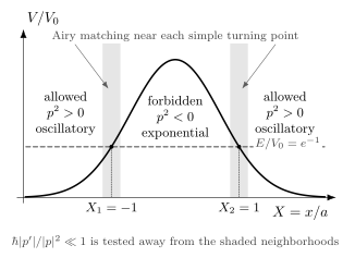
In the dimensionless coordinate $X=x/a$, consider the smooth barrier $V/V_0=e^{-X^2}$ at $E/V_0=e^{-1}$. The exact simple turning points are $X=-1$ and $X=1$. Leading WKB is oscillatory where $p^2\gt0$ and exponential where $p^2\lt0$, but it is nonuniform in the shaded turning-point neighborhoods, where Airy matching is required. Exact regime geometry for the displayed model; neighborhood widths schematic.

Tong develops the semiclassical expansion, local validity test, and Airy matching in Tong 2017, §2.2, printed pp. 37–49.

Exact discontinuous-barrier check

Let $V=V_0$ on $0\lt x\lt d$, let $V=0$ outside, and take $0\lt E\lt V_0$. For this finite step, continuity of $\psi$ and $\psi'$ at $x=0$ and $x=d$ fixes the reflection and transmission amplitudes. Direct interface matching gives

$$T_{\rm exact} =\left[ 1+\frac{V_0^2\sinh^2(\kappa d)}{4E(V_0-E)} \right]^{-1}, \qquad \kappa=\frac{\sqrt{2M(V_0-E)}}{\hbar}.$$

For $\kappa d\gg1$,

$$T_{\rm exact} \simeq \frac{16E(V_0-E)}{V_0^2}e^{-2\kappa d}.$$

The WKB action reproduces the decisive exponent $e^{-2\int_0^d\kappa dx}=e^{-2\kappa d}$, but not the sharp-interface prefactor. The barrier edges are discontinuous interfaces, not smooth simple turning points, so they require direct matching rather than an Airy patch. Tong obtains the exact coefficient and thick-barrier limit in Tong, Quantum Mechanics, undated, §2.4.2, printed pp. 60–62. Tong places the interfaces at $x=\pm a_{\rm T}$, so the width used here is $d=2a_{\rm T}$; his $e^{-4\kappa a_{\rm T}}$ is therefore the same exponent.

Common pitfalls

Calling a dimensionful number small. A coupling or derivative becomes a control only after comparison with the relevant gap, time, norm, or wavelength scale.

Confusing weak with short-lived. A weak resonant perturbation can produce an order-one transition after a sufficiently long time.

Confusing slow with gapped. Smooth slow driving can still violate a simple adiabatic approximation when the band gap closes.

Continuing WKB through a turning point. The outer expansion is nonuniform there. A local matching problem, and sometimes global Stokes data, is required.

The bounded bridge to gravitation

For a self-adjoint stationary mode problem, spectral perturbation can control weak changes when the relevant eigenvalue remains isolated. For a high-frequency field on a slowly varying geometry, covariant geometric optics is governed by wavelength-to-background-scale ratios and the field equation’s principal symbol; it is not literally the one-dimensional Schrödinger WKB formula.

Likewise, gapped self-adjoint adiabatic theorems do not directly govern outgoing black-hole resonances or quasinormal modes. Non-self-adjoint spectral problems can require left and right modes, pole perturbation, and separate control of boundary conditions. Weak coupling, slow evolution, and short wavelength must therefore be checked independently.

Continue with Density Operators, Entanglement, and Reduced States.

Exercises

Match each regime to its control

For each situation below, identify the approximation and write the dimensionless diagnostic that must be checked:

1. A static level $n$ is weakly mixed with a level $m$ separated by $\Delta_{mn}=|E_m^{(0)}-E_n^{(0)}|$.
2. A bounded interaction-picture perturbation satisfies $\lVert V_I(t)\rVert\le V_*$ for a duration $T$.
3. A band is driven along $s\in[0,1]$ in time $\tau$, with minimum exterior gap $g_{\min}$ and $\max_s|\langle m|\partial_sH|n\rangle|\le M_{mn}$.
4. A stationary wave has real local momentum $p(x)$ away from isolated zeros.

State one failure boundary that the diagnostic alone cannot cross.

Solution

1. Stationary perturbation uses $\epsilon_{mn}^{\rm stat}=|\lambda V_{mn}|/\Delta_{mn}$. Degeneracy or a sufficiently small denominator requires diagonalization in the affected subspace; in infinite dimension, one must also control the sum and domains.
2. Time-dependent perturbation has the sufficient bound $\eta_{\rm TD}\le |\lambda|V_*T/\hbar$. Near a resonant matrix element, the explicit first-order amplitude must also remain small, for example $|\lambda v|T/(2\hbar)\ll1$ in the cosine drive above. Reaching order one calls for resummation or exact driven dynamics rather than a first-order truncation.
3. The elementary adiabatic ratio obeys $\epsilon_{mn}^{\rm ad}\le\hbar M_{mn}/(\tau g_{\min}^2)$. A closing gap invalidates this estimate, and a theorem additionally needs its stated differentiability, domain, and spectral hypotheses.
4. WKB requires at least $\epsilon_{\rm WKB}=\hbar|p'|/|p|^2\ll1$, together with control of the residual involving $p''$. It fails at a turning point $p=0$ and needs a separate local matching problem there.

WKB flux on both sides of a turning region

For an allowed-region branch $\psi_+=C p^{-1/2}e^{i\int p(x')\,dx'/\hbar}$, calculate the probability current through leading order. Then show that a pure real decaying branch $D\kappa^{-1/2}e^{-\int\kappa dx}$ in a forbidden region carries zero current. Explain why this does not say that every superposition of growing and decaying branches has zero current.

Solution

Differentiating the allowed branch gives

$$\psi_+'= \left(-\frac{p'}{2p}+\frac{ip}{\hbar}\right)\psi_+.$$

The amplitude-derivative term is real in $\psi_+^*\psi_+'$, so

$$j=\frac{\hbar}{M}\operatorname{Im}(\psi_+^*\psi_+') =\frac{\hbar}{M}\frac{|C|^2}{p}\frac{p}{\hbar} =\frac{|C|^2}{M}.$$

For the pure decaying forbidden branch with a constant overall phase, $\psi^*\psi'$ is real, hence $j=0$. A linear combination of growing and decaying branches can have a relative complex phase; its cross term can then carry nonzero current. Barrier transmission is determined only after the global boundary and matching conditions select that combination.

References

• Jansen, Sabine, Mary-Beth Ruskai, and Ruedi Seiler. “Bounds for the Adiabatic Approximation with Applications to Quantum Computation.” Journal of Mathematical Physics 48 (2007): 102111. doi:10.1063/1.2798382. Open PDF.
• Tong, David. Quantum Mechanics, §2.4.2, printed pp. 60–62. Cambridge lecture notes, undated; official PDF inspected August 30, 2026. Official PDF.
• Tong, David. Topics in Quantum Mechanics, §2.2, printed pp. 37–49. Cambridge lecture notes, 2017. Official PDF.
• Turner, Andrew. Quantum Theory I, Lecture 8, prepared for instructor Senthil Todadri, MIT 8.321, Fall 2017, printed pp. 42–43. MIT OpenCourseWare PDF.