Proper Time, Worldlines, and the Clock Effect

The elapsed times of two ideal clocks are determined by the Lorentzian lengths of their two worldlines between common departure and reunion events. For each future-directed timelike path $\gamma$, compute $\tau[\gamma]$ and compare the results. Acceleration matters only insofar as it changes the path; “acceleration causes less aging” is neither the formula nor a generally valid explanation.

Required background. Calculus and Linear Algebra provides parameterized curves and line integrals; Variational Mechanics and Symmetries supplies functionals, endpoint conditions, and the distinction between an extremum and a merely stationary path.

The worldline functional

Let a piecewise-smooth future-directed timelike worldline be $x^\mu(\lambda)$, where $\lambda$ is any increasing parameter. Its proper time is

$$\tau[\gamma] =\int_{\lambda_1}^{\lambda_2} \sqrt{-\eta_{\mu\nu} \frac{dx^\mu}{d\lambda} \frac{dx^\nu}{d\lambda}}\,d\lambda.$$

The expression is invariant under Lorentz transformations and under smooth reparametrization of the same oriented path. In any inertial coordinates with $t$ as parameter,

$$d\tau=dt\sqrt{1-|\mathbf v(t)|^2} =\frac{dt}{\gamma(t)}, \qquad \mathbf v=\frac{d\mathbf x}{dt}.$$

Thus an ideal clock measures a scalar accumulated locally along its own trajectory, not a global coordinate time. Tong derives these formulas in Tong 2013, §7.4.1, printed pp. 133–134 (PDF); the parameter-independent form also appears in Tong, General Relativity, §1.2.1, Eq. (1.16).

Why the inertial path has the most proper time

Take two timelike-separated events $A$ and $B$. There is an inertial frame in which they occur at the same spatial position, say at $t=0$ and $t=T$. The straight inertial worldline has $\mathbf v=0$ and proper time $T$. Any other future-directed timelike worldline between them satisfies

$$\tau =\int_0^T\sqrt{1-|\mathbf v(t)|^2}\,dt \le\int_0^Tdt=T,$$

with equality only when $\mathbf v=0$ almost everywhere. This proves, in flat spacetime, that the straight timelike segment maximizes proper time between fixed endpoints. Hughes 2024, Lecture 16, §16.4, printed pp. 133–134, Eqs. (16.25)–(16.30) (PDF) independently derives inertial motion as the variational extremal; the inequality above supplies the stronger global maximum statement used here.

The inequality is geometric. One clock need not remain “really at rest,” because rest is frame-dependent. What distinguishes the clocks is that their complete worldlines are different: one is the straight segment, the other is not.

Worked clock comparison

Earth and a spacecraft meet at event $A$. In Earth’s inertial frame, the spacecraft travels outward for $5$ years at speed $v=3/5$, reverses direction over an idealized negligible interval, and returns at the same speed, meeting Earth at event $B$ after $10$ Earth years. What do the two clocks read?

Solution

Earth follows $\mathbf x=0$, so

$$\tau_{\rm E}=\int_0^{10}dt=10\ {\rm yr}.$$

On both constant-speed spacecraft legs,

$$\sqrt{1-v^2} =\sqrt{1-\frac9{25}} =\frac45.$$

The spacecraft clock therefore accumulates

$$\tau_{\rm ship} =2\int_0^5\frac45\,dt =8\ {\rm yr}.$$

The clock effect is

$$\Delta\tau=\tau_{\rm E}-\tau_{\rm ship}=2\ {\rm yr}.$$

Both values are worldline integrals between the same events, so every coordinate system yields the same comparison. The instantaneous reversal is a calculational idealization. Replacing it by a smooth finite-acceleration arc adds that arc’s proper-time integral and approaches the result above as its duration becomes small. Acceleration identifies and constructs the bent path; it is not an extra aging term in the integrand.

Why reciprocal time dilation is consistent

On either straight leg, the spacecraft can use a comoving inertial clock lattice and regard Earth as moving. But the outward and return lattices have different simultaneity planes. They cannot be joined by pretending that the same distant Earth event remains simultaneous with the turnaround.

At turnaround $C=(t,x)=(5\ {\rm yr},3\ {\rm ly})$, the inertial frame moving outward at $v=3/5$ assigns simultaneous events by $t-vx=\text{constant}$. Its simultaneous Earth event has

$$t_{{\rm E,out}}=5-\frac35\,3=3.2\ {\rm yr}.$$

The return frame moves at $-v$ and uses $t+vx=\text{constant}$, giving

$$t_{{\rm E,in}}=5+\frac35\,3=6.8\ {\rm yr}.$$

Each leg lasts $4$ spacecraft years. Reciprocal time dilation assigns Earth $4/\gamma=3.2$ years during each leg, but changing the distant-simultaneity convention adds a $6.8-3.2=3.6$ year reassignment. The total is $3.2+3.6+3.2=10$ Earth years. No clock jumps and no signal travels instantaneously: the reassignment concerns which distant event the traveler calls “now,” not which light arrives at the ship. A smooth turnaround makes the reassignment continuous. This resolves the apparent reciprocity puzzle using the same clock integral as before; compare Tong 2013, §7.2.3, pp. 119–122, PDF.

Inspect the two worldlines first in the diagram, then the two simultaneity lines through the turnaround. Both clocks share $A$ and $B$, but only the spacecraft changes inertial frames.

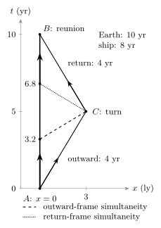
For $v=3c/5$ and a ten-year Earth-frame journey, Earth records ten years and the ship eight. Dashed and dotted lines assign different Earth events as simultaneous with the turnaround; they are not light signals. The 1+1 diagram uses equal scales for years and light-years and idealizes an instantaneous reversal.

Interpretation and limits

• In a chosen inertial frame, a constant-speed leg accumulates $d\tau=dt/\gamma\lt dt$ even where proper acceleration vanishes. This local rate statement is not by itself a two-clock comparison; the invariant comparison uses complete worldlines with common endpoints.
• A short smooth turnaround arc contributes only its own proper-time integral. The magnitude of proper acceleration is not an additional term in the integrand.
• Null curves have $d\tau=0$ and cannot carry a massive ideal clock or define a photon rest frame.
• A comparison of readings at specified separated events is well defined, but choosing which distant events count as simultaneous requires an additional convention. It is not the invariant common-departure-and-reunion comparison calculated here.
• The ideal-clock hypothesis neglects engineering sensitivity to acceleration. In curved spacetime the same local integral uses $g_{\mu\nu}(x)$, and gravity changes which worldlines are available and extremal.

The normalization check is immediate: for a clock instantaneously at rest, $d\tau=dt$; as $|\mathbf v|\to1$, $d\tau/dt\to0$. Restoring $c$ changes the square root to $\sqrt{1-v^2/c^2}$.

Four-Vectors and Lorentz-Invariant Decomposition now turns the tangent $dx^\mu/d\tau$ into a four-vector and formalizes observer-dependent projections.

References

• Hughes, Scott A. Introduction to Relativity and Spacetime Physics. MIT 8.033 Lecture 16, especially §16.4, printed pp. 133–134 (PDF), Fall 2024.
• Tong, David. Dynamics and Relativity. §7.2.3, pp. 119–122, and §7.4.1, “Proper Time,” pp. 133–134, PDF, University of Cambridge, Lent Term 2013. Signature translated from $(+---)$ to $(-+++)$.
• Tong, David. General Relativity. §1.2.1, “A Particle in Minkowski Spacetime,” especially Eq. (1.16), University of Cambridge.