Reissner–Nordström Horizons and Extensions

The Reissner–Nordström metric changes its global causal architecture when its two radial roots are distinct, coincident, or absent. A nonzero subextremal charge produces an infinite analytic chain separated by outer and inner horizons; exact extremality produces a different degenerate-horizon extension with an internal infinity and no bifurcation sphere; superextremality leaves one static, horizonless domain with a naked timelike singularity. The neutral endpoint is Schwarzschild, not a two-horizon diagram with the inner labels erased.

This page starts from the exact metric and electromagnetic field and constructs the charts needed to interpret those statements. It concerns the ideal four-dimensional, asymptotically flat Einstein–Maxwell background with $M\gt0$ and $\Lambda=0$. It does not claim that the inner horizon is stable, that a superextremal solution forms from regular data, or that the eternal extension is the spacetime of a collapsing star.

Required background. The Einstein Equation supplies the governing field equation; the preceding Reissner–Nordström page supplies the metric-field solution being extended.

Helpful background. Exact Solutions of Einstein’s Equations compares this spacetime with other exact solutions; Causality and Global Structure supplies the global language; The Riemann Curvature Tensor supports the invariant test; Spacetime Extensions and Maximality distinguishes analytic continuation from geodesic completeness; and Affine and Variational Geodesics supports the crossing tests.

Roots, horizons, and what local algebra proves

Write $Q^2=Q_e^2+Q_m^2$. In the normalization established on the preceding page,

$$ds^2=-f(r)\,dt^2+\frac{dr^2}{f(r)}+r^2d\Omega_2^2, \qquad f(r)=1-\frac{2GM}{r}+\frac{GQ^2}{r^2} =\frac{(r-r_+)(r-r_-)}{r^2},$$

where

$$r_\pm=GM\pm\sqrt{G^2M^2-GQ^2}.$$

The discriminant classifies the positive-radius zeros, but a zero of $f$ is only the beginning of the geometric argument. In a regular chart, the stationary Killing field becomes null and normal to each positive zero, so the zero is a Killing horizon. A double zero is degenerate: its surface gravity vanishes for the asymptotically normalized Killing field. An event horizon is instead the global boundary $\partial J^-(\mathscr I^+)$ relative to a chosen asymptotic end, while a Cauchy horizon bounds the domain determined by specified initial data. The corresponding definitions are developed on Killing Horizons, Event Horizons as Global Boundaries, and Cauchy Horizons and Their Generators.

Parameters	Positive-radius roots	Sign of $f$	Immediate consequence
$0\lt Q^2\lt GM^2$	Two simple roots $0\lt r_-\lt r_+$	Positive outside the roots; negative between them	Two distinct Killing-horizon radii and a nonstatic band
$Q^2=GM^2$	One double root $r_0=GM$	Nonnegative on both sides	One degenerate radius and no trapped band
$Q^2\gt GM^2$	No real root	Positive for every $r\gt0$	One static horizonless domain
$Q=0$	Only $r_+=2GM$	Schwarzschild sign pattern	The formal $r_-=0$ factor cancels and is not a horizon

For a simple root $r_h$, define the signed quantity

$$\kappa_h=\frac12 f'(r_h), \qquad \kappa_+=\frac{r_+-r_-}{2r_+^2}\gt0, \qquad \kappa_- =\frac{r_--r_+}{2r_-^2}\lt0.$$

The sign on $\kappa_-$ is useful in the coordinate construction; references that quote a positive inner-horizon surface gravity usually mean $|\kappa_-|$. For the mechanics of these horizons, see Black-Hole Geometry.

The normalized plot shows the same transition twice. Here $|Q|$ means $\sqrt{Q_e^2+Q_m^2}$. First follow the two root loci into their extremal merger, then compare how the radial profiles cross, touch, or remain positive.

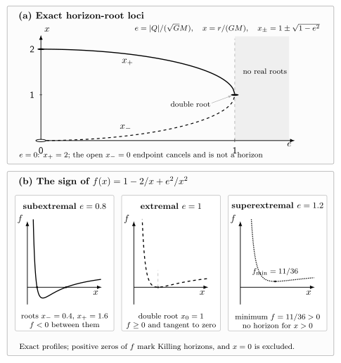
For $M\gt0$, normalized charge $e=|Q|/(\sqrt{G}M)$ gives horizon roots $x_\pm=1\pm\sqrt{1-e^2}$, with $x=r/(GM)$. Two positive roots exist for $0\lt e\lt1$, they merge at $x=1$ when $e=1$, and no real roots remain for $e\gt1$; at $e=0$ the formal $x_-=0$ endpoint cancels and is not a horizon. Exact profiles at $e=0.8$, $1$, and $1.2$ show roots $0.4$ and $1.6$ with $f\lt0$ between them, a double tangent root, and a positive minimum $f=11/36$ at $x=1.44$. Only positive zeros mark Killing horizons, and $x=0$ is excluded. Every curve is quantitative in the displayed normalized coordinates.

Crossing a simple horizon

Assume $0\lt Q^2\lt GM^2$ and define the tortoise coordinate by $dr_*/dr=f^{-1}$. Partial fractions give

$$r_*=r +\frac{r_+^2}{r_+-r_-}\ln\left|\frac{r}{r_+}-1\right| -\frac{r_-^2}{r_+-r_-}\ln\left|\frac{r}{r_-}-1\right|.$$

This expression defines $r_*$ separately on the three open intervals cut by the roots. Its additive constant may be chosen independently in each chart; no single real logarithm crosses either root.

Differentiation is the quickest check. Near either simple root,

$$r_*=\frac{1}{2\kappa_h}\ln|r-r_h|+\text{a function regular at }r_h.$$

Set $v=t+r_*$ for an advanced chart. Since $dt=dv-dr/f$,

$$ds^2=-f\,dv^2+2\,dv\,dr+r^2d\Omega_2^2.$$

The $(v,r)$ block has determinant $-1$ and inverse

$$g^{AB}=\begin{pmatrix}0&1\\[2pt]1&f\end{pmatrix}.$$

It is therefore nondegenerate at both root radii. At $f=0$, the normal vector to $r=\text{constant}$ is $g^{ar}\partial_a=\partial_v$, exactly the Killing generator; this verifies the local Killing-horizon claim without treating the singular static chart as evidence.

The electromagnetic field crosses with the geometry:

$$F=\frac{Q_e}{r^2}\,dr\wedge dv +Q_m\sin\theta\,d\theta\wedge d\phi.$$

The future-regular electric potential $A_e=-Q_e\,dv/r$ differs from the transformed static potential by the exact radial term $Q_e\,dr/(rf)$ on each overlap interval. The magnetic field retains the north/south angular gauge patches constructed on the preceding page. Thus a bad choice of potential is not a singularity of $F$.

Advanced and retarded coordinates cover complementary null branches but do not contain the full maximal extension. At the outer root relative to the selected exterior, finite $v$ crosses the future branch and finite $u=t-r_*$ crosses the past branch. That shortcut does not apply globally at the inner root: the two branches bounding the future of one trapped block are both future Cauchy-horizon branches, even though one is reached in an advanced chart and the other in a retarded chart. Neither one-sided chart contains a bifurcation two-sphere. To include both branches near one selected simple horizon, choose

$$U_h=-e^{-\kappa_h u}, \qquad V_h=e^{\kappa_h v}.$$

Quadrant signs are changed when adjoining neighboring blocks. The radial metric becomes

$$ds^2_{(2)} =-\frac{f}{\kappa_h^2}e^{-2\kappa_h r_*}\,dU_h\,dV_h.$$

Because $f=2\kappa_h(r-r_h)+O((r-r_h)^2)$ and

$$e^{-2\kappa_h r_*} =C_h|r-r_h|^{-1}\left[1+O(r-r_h)\right], \qquad C_h\gt0,$$

the radial coefficient tends one-sidedly to $-(2C_h/\kappa_h)\operatorname{sgn}(r-r_h)$, which is finite and nonzero. The constant $C_h$ records the additive choice in $r_*$ and the selected side; it has no invariant significance. A horizon-shifted potential $-Q_e(1/r-1/r_h)dt$ is likewise regular because its coefficient vanishes linearly. The scale $\kappa_+$ does not regularize $r_-$, and $\kappa_-$ does not regularize $r_+$: the logarithmic residues $1/(2\kappa_\pm)$ are unequal and have opposite signs. The maximal subextremal solution therefore uses overlapping root-adapted patches, as constructed in Graves and Brill 1960, § III, printed pp. 1510–1511, Eqs. (21)–(27).

The displayed sign is a one-sided coordinate convention, not a jump in the metric. When adjoining the neighboring quadrant, reverse the sign of one of $U_h,V_h$ so that $U_hV_h$ is proportional to $r-r_h$, rather than $|r-r_h|$. The corresponding sign reversal of $dU_h\,dV_h$ cancels the $\operatorname{sgn}(r-r_h)$ above. Choosing the independent additive constants in $r_*$—equivalently, the constant scales of $U_h$ and $V_h$—to agree on the overlap then makes the two one-sided expressions meet with one finite nonzero analytic coefficient. This is the local matching step that turns two horizon-regular sides into one chart.

At $Q=0$, the two-root expression should not be used with $r_-=0$. After cancellation, the correct Schwarzschild antiderivative is $r_*=r+2GM\ln|r/(2GM)-1|$, up to an additive constant.

The double root is a different coordinate problem

At exact extremality, $r_0=GM$ and

$$f=\left(1-\frac{r_0}{r}\right)^2, \qquad r_*=r+2r_0\ln\left|\frac{r}{r_0}-1\right| -\frac{r_0^2}{r-r_0}.$$

The pole in $r_*$ replaces the simple-root logarithm. Since $f'(r_0)=0$, no nonzero exponential scale $\kappa_h$ exists; the nonextremal Kruskal coordinates degenerate as $r_+\to r_-$. Nevertheless, $v=t+r_*$ again gives the smooth advanced metric above and crosses one future component of the double horizon. Coordinate regularity survives even though the limiting nonextremal coordinates do not.

The phrase “infinite throat” refers to a particular spatial slice. For $r_2\gt r_1\gt r_0$, its radial proper length is

$$\ell(r_1,r_2) =r_2-r_1+r_0\ln\!\left(\frac{r_2-r_0}{r_1-r_0}\right),$$

which diverges as $r_1\downarrow r_0$. A causal traveler is different. For a radial timelike geodesic with conserved energy $E\ne0$,

$$\dot r^2=E^2-f\longrightarrow E^2 \qquad (r\to r_0),$$

so any such geodesic that reaches the horizon crosses it in finite proper time. In advanced coordinates, the ingoing null field $k=-\partial_r$ is regular, null, geodesic, and affinely parametrized because every $\Gamma^a{}_{rr}$ vanishes. Infinite distance within the static slice is not causal inaccessibility.

On the horizon, $\xi=\partial_v$ obeys $\xi^b\nabla_b\xi^a=\kappa\xi^a=0$, so $v$ is an affine parameter along each generator. In the standard extremal extension, the horizon has no bifurcation two-sphere: toward the past, $v\to-\infty$, its generators have infinite affine length rather than meeting at a finite bifurcation surface. They instead run to an internal infinity approached rather than intersected by the static slices. This extremal topology is described in Bičák 2000, § 3.2, printed p. 39, Eq. (19) and the following paragraph, Open PDF; the directly constructed canonical graph and its additional primary sources are recorded on Reissner–Nordström Conformal Diagrams. The global distinction is another reason not to obtain extremal spacetime by merely squeezing the two subextremal horizon lines together.

Analytic blocks and causal boundaries

Here an analytic block means a connected radial orbit-space region between consecutive horizon, singular, or conformal boundaries. A maximal analytic extension admits no proper analytic isometric extension into a larger connected Einstein–Maxwell spacetime. In the standard construction, adjoining root-adapted blocks across every regular horizon branch produces the full infinite chain, whose remaining ends are conformal infinities or the curvature-singular $r=0$ boundaries. This object is not the same as the maximal globally hyperbolic development of initial data.

In the strict subextremal extension, the sign of $f=g^{ab}(\nabla_a r)(\nabla_b r)$ supplies a coordinate-independent causal check. The same classification can be read from the two future-directed radial null normals in an advanced block:

$$\ell=\partial_v+\frac{f}{2}\partial_r, \qquad n=-\partial_r, \qquad g(\ell,n)=-1.$$

The time orientation is anchored in the selected exterior, not inferred from the sign of $f$. There $\partial_v$ is future timelike and

$$g(\ell,\partial_v)=-\frac f2\lt0, \qquad g(n,\partial_v)=-1\lt0,$$

so both null normals are future-directed. Continuity across the future outer horizon fixes that orientation in the adjacent future block; its time reverse requires the oppositely oriented construction.

For a symmetry sphere of area $4\pi r^2$, their null expansions are

$$\theta_{(\ell)}=\frac{1}{4\pi r^2}\mathcal L_\ell(4\pi r^2) =\frac{f}{r}, \qquad \theta_{(n)}=\frac{1}{4\pi r^2}\mathcal L_n(4\pi r^2) =-\frac{2}{r}.$$

Positive rescalings of $\ell$ and $n$ change their magnitudes but preserve these signs and zeros. Thus an exterior has one positive and one negative expansion, a future block with $f\lt0$ has both negative and is trapped, and its time reverse is anti-trapped. At a horizon $\theta_{(\ell)}=0$; deciding whether that marginal surface belongs to an event horizon or a Cauchy horizon still requires the global information below.

Radial interval	Causal character	Role in the ideal extension
$r\gt r_+$	$\partial_t$ timelike; $\nabla r$ spacelike	Static asymptotically flat exterior
$r_-\lt r\lt r_+$	$\partial_t$ spacelike; $\nabla r$ timelike	Future black-hole sectors are trapped; their time reverses are anti-trapped
$0\lt r\lt r_-$	$\partial_t$ timelike; $\nabla r$ spacelike	Static inner block bounded by Cauchy horizons and timelike singularities

Crossing successive outer and inner branches with the two root-adapted charts produces an infinite chain of asymptotically flat ends, nonstatic bands, and static inner blocks. The future outer branch adjoining a chosen exterior is an event-horizon branch for that end; the past outer branch adjoining that same exterior is its white-hole counterpart. In the many-ended analytic extension, these adjoining branches are not necessarily the entire global boundaries: those require specifying the asymptotic end or ends and tracing their causal past or future. An inner branch is a Cauchy horizon relative to the chosen partial Cauchy surface. Data on that surface determine the maximal globally hyperbolic development only up to this boundary. The exact analytic Reissner–Nordström solution supplies a continuation beyond it, but that continuation is additional global information rather than a prediction fixed by the partial Cauchy data Bičák 2000, § 3.1, printed pp. 34–35, especially p. 35, Open PDF.

Since $f\gt0$ near $r=0$, the limiting $r=\text{constant}$ hypersurfaces are timelike, and the invariant

$$R_{\mu\nu}R^{\mu\nu}=\frac{4G^2Q^4}{r^8}$$

shows that $r=0$ is a curvature-singular boundary rather than another removable seam. It is also reached in finite affine parameter. On any regular radial interval, conservation of $E=f\,dt/d\lambda$ and the null condition give

$$\left(\frac{dr}{d\lambda}\right)^2=E^2.$$

Consequently a radial null geodesic directed from $r=r_1$ to the singularity has affine length $\Delta\lambda=r_1/|E|$. The horizon-regular charts continue this geodesic across the roots, but no chart continues it through the curvature blow-up. The maximal analytic extension is therefore geodesically incomplete: “maximal” does not mean “complete.” Bičák gives the ideal chain and its boundary labels in Bičák 2000, § 3.1, printed pp. 32–34, Eq. (11) and Fig. 5, Open PDF.

The following page, Invariants, Singularities, and Controlled Limits, compares this Ricci-square test with the Weyl and Kretschmann invariants and develops the extremal near-horizon limit.

The root plot answers where the horizons can occur; the conformal diagrams answer how the resulting blocks meet. Compare the trapped band and separate horizon radii in the first panel with the absence of both the trapped band and the bifurcation sphere in the extremal panel, then with the single superextremal domain. The canonical diagram uses geometrized notation $m\equiv GM$ and $q^2\equiv GQ^2=G(Q_e^2+Q_m^2)$; hence its extremal label $r=m$ means $r=r_0=GM$, and $c^0$ denotes the cylindrical internal infinity. In the extremal graph, the event- and Cauchy-horizon components remain globally distinct even though both have this same radius, and the degenerate blocks still repeat. The complete boundary key remains on Reissner–Nordström Conformal Diagrams.

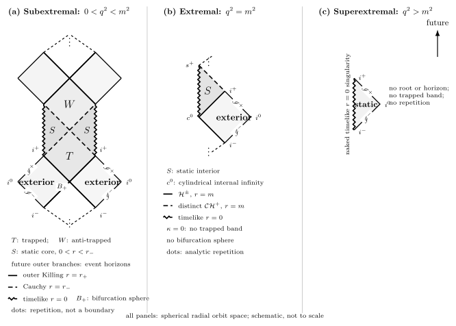
Charge separates the exact Reissner–Nordström family into three causal graphs: an infinitely repeating subextremal extension with outer and inner horizons, a distinct extremal extension with a degenerate horizon and no bifurcation sphere, and a horizonless superextremal spacetime with a naked timelike singularity. Future points upward; each spherical radial diagram is schematic and not to scale.

The smooth inner horizons in this diagram belong to the exact stationary solution. Reissner–Nordström and Kerr Interiors explains their blueshift and nonlinear fate; the diagram alone does not establish their stability.

Horizonless and nonuniform limits

In the superextremal regime, the normalized lapse $f(x)=1-2/x+e^2/x^2$ has its minimum at $x=e^2$, where $f_{\min}=1-e^{-2}\gt0$. There is no horizon chart boundary and no second analytic block. Radial null geodesics satisfy $dr/d\lambda=\pm E$, so they reach the timelike singular boundary in finite affine parameter; outgoing ones place that boundary in the causal past of future null infinity. “Naked” describes this exact causal relation, not a formation theorem or a verdict on cosmic censorship.

Take the neutral limit at fixed $M\gt0$. In advanced Eddington–Finkelstein coordinates, the metric coefficients converge in $C^\infty$ on every compact subset of $r\gt0$; the diagonal static coefficient $g_{rr}=f^{-1}$ is not a common regular representative at the limiting Schwarzschild horizon. The root expansions are

$$r_-=\frac{Q^2}{2M}+O\!\left(\frac{Q^4}{GM^3}\right), \qquad r_+=2GM-\frac{Q^2}{2M}+O\!\left(\frac{Q^4}{GM^3}\right).$$

Thus the metric tends smoothly to Schwarzschild in that common regular chart on every domain $r\ge\epsilon\gt0$, while the Cauchy horizon and inner static blocks collapse into the central region. At fixed $M\gt0$, the extremal limit $Q^2\uparrow GM^2$ is nonuniform in another way: $r_+-r_-=2\sqrt{G^2M^2-GQ^2}$ and $\kappa_+\to0$, so both the throat and the coordinate scale change. Algebraic convergence of $f$ does not imply convergence of the maximal diagrams.

Common pitfalls

Calling every zero an event horizon. The equation $f=0$ identifies a Killing horizon after regular extension. Event-horizon and Cauchy-horizon labels require global causal data and a specified asymptotic end or data surface.

Treating one regular chart as maximal. Advanced and retarded coordinates cross complementary null branches, but their future/past labels depend on the root and analytic block. A maximal extension needs their root-adapted overlaps and must admit no proper analytic continuation.

Reading the extremal throat as an obstruction to infall. The divergent length belongs to a static spacelike slice. Regular null and timelike curves cross the horizon in finite affine or proper parameter.

Confusing an exact extension with a stable interior. Analytic continuation answers a geometric background question. Perturbative blueshift, mass inflation, collapse, and censorship require dynamics beyond this page.

Treating continuation beyond a Cauchy horizon as Cauchy prediction. The exact solution supplies a smooth analytic continuation, but data on the chosen partial Cauchy surface determine only its maximal globally hyperbolic development. Extra assumptions are needed to select what, if anything, lies beyond that development’s Cauchy horizon.

Reading “maximal” as “complete.” Maximal analytic extension means that no larger connected analytic Einstein–Maxwell spacetime contains this one as a proper open subspacetime. Radial null geodesics still reach the curvature singularity at $r=0$ in finite affine parameter, so the maximal extension is geodesically incomplete.

Exercises

1. Roots, signs, and the neutral endpoint

Factor $r^2f$ and prove the four rows of the regime table. Explain why $r_-=0$ at $Q=0$ is not a horizon.

Solution

The quadratic $r^2-2GMr+GQ^2$ has discriminant $4(G^2M^2-GQ^2)$ and roots $r_\pm$. For two distinct positive roots, the upward-opening numerator is positive outside them and negative between them; division by $r^2\gt0$ preserves the signs. A double root gives $f=(1-GM/r)^2\ge0$, while a negative discriminant leaves the numerator positive. At $Q=0$, $r^2f=r(r-2GM)$, so one factor of $r$ cancels against the denominator: $f=1-2GM/r$ on $r\gt0$, and only $2GM$ is a zero.

2. Check the two logarithmic residues

Differentiate the subextremal $r_*$ and show that $dr_*/dr=f^{-1}$. Then show that the coefficient of $\ln|r-r_h|$ is $1/(2\kappa_h)$ at each root.

Solution

Using $r_++r_-=2GM$ and $r_+r_-=GQ^2$, differentiation gives

$$1+\frac{r_+^2}{(r_+-r_-)(r-r_+)} -\frac{r_-^2}{(r_+-r_-)(r-r_-)} =\frac{r^2}{(r-r_+)(r-r_-)}=\frac1f.$$

At $r_+$ the residue is $r_+^2/(r_+-r_-)=1/(2\kappa_+)$. At $r_-$ it is $-r_-^2/(r_+-r_-)=1/(2\kappa_-)$. These different signed residues require distinct root-adapted exponential rates; one rate cannot regularize both roots.

3. Transform the metric and the field

Starting with $v=t+r_*$, derive the advanced metric and Maxwell two-form. Verify that their radial components remain finite at $f=0$.

Solution

Substitute $dt=dv-dr/f$ into $-fdt^2+dr^2/f$; the $dr^2/f$ terms cancel, leaving $-f\,dv^2+2\,dv\,dr$. Its determinant is $-1$. Since $dr\wedge dt=dr\wedge(dv-dr/f)=dr\wedge dv$, the electric field becomes $Q_e\,dr\wedge dv/r^2$; the magnetic term is unchanged. Both coefficients are finite at every positive root. The potential $-Q_e\,dv/r$ is regular across the corresponding future branch.

4. Infinite spatial distance, finite causal crossing

For extremal $f=(1-r_0/r)^2$, verify the displayed proper length and show directly that $k=-\partial_r$ is an affinely parametrized ingoing null geodesic in the advanced chart.

Solution

On the exterior static slice, $f^{-1/2}=r/(r-r_0)$, whose integral is $r+r_0\ln(r-r_0)$ up to a constant; taking the difference between $r_1$ and $r_2$ gives the displayed $\ell$, which diverges as $r_1\downarrow r_0$. In $(v,r)$ coordinates, $dv=0$ makes $ds^2=0$. The metric components $g_{rr}=0$ and $g_{vr}=1$ are constant in $r$, so $\Gamma^a{}_{rr}=0$. Hence $k^b\nabla_bk^a=0$, and $\lambda=-r$ is an affine parameter increasing toward the future along $k=-\partial_r$ across $r_0$.

5. Which horizon is which?

Classify the future and past outer-horizon branches adjoining one selected asymptotically flat exterior and the inner branches at $r=r_-$. Then list the block types followed by an ideal future-directed causal curve that traverses the repeating subextremal extension without meeting $r=0$. Why does the extremal double root not erase the distinction between event- and Cauchy-horizon components?

Solution

Every smooth branch at either positive simple root is a Killing horizon of $\partial_t$. The future outer branch adjoining the selected exterior belongs to $\partial J^-(\mathscr I^+)$ for that end; the past outer branch adjoining the same exterior is its white-hole counterpart. Neither statement identifies the entire global boundary in the many-ended extension. The inner branches are future or past Cauchy horizons relative to the chosen partial Cauchy surface, because they bound the region uniquely determined by those data.

Starting in an exterior, a traversing future-directed curve crosses a future outer branch into a trapped band, then an inner Cauchy horizon into a static inner block. If it avoids the timelike singularity and crosses the next inner branch, it enters an anti-trapped band; crossing the next outer branch reaches another asymptotically flat exterior. The pattern then repeats in the ideal analytic solution. At extremality, root multiplicity says that the local Killing horizon is degenerate, but it does not determine global causal roles: distinct null components at the same radius can still bound $J^-(\mathscr I^+)$ and a domain of dependence, respectively. The extremal diagram has no bifurcation sphere connecting them.

6. Diagnose trapped spheres and affine incompleteness

In the advanced metric, verify that $\ell=\partial_v+(f/2)\partial_r$ and $n=-\partial_r$ are null with $g(\ell,n)=-1$. Derive their expansions and use a radial null geodesic to explain why the maximal analytic extension is nevertheless incomplete.

Solution

From $ds^2_{(2)}=-f\,dv^2+2\,dv\,dr$,

$$g(\ell,\ell)=-f+2\left(\frac f2\right)=0, \qquad g(n,n)=0, \qquad g(\ell,n)=-1.$$

For any radial null normal $k$, the sphere expansion is the fractional rate of change of its area:

$$\theta_{(k)}=\frac{1}{4\pi r^2}\mathcal L_k(4\pi r^2) =\frac{2k(r)}{r}.$$

Therefore $\theta_{(\ell)}=f/r$ and $\theta_{(n)}=-2/r$. In a future block between two simple roots, $f\lt0$, so both are negative and the spheres are trapped. Outside that band their signs are opposite; at a root $\theta_{(\ell)}=0$.

For a radial null geodesic, $E=f\,dt/d\lambda$ and $0=-f\dot t^2+\dot r^2/f$ imply $\dot r^2=E^2$. Once directed toward the centre from radius $r_1$, it reaches $r=0$ after $\Delta\lambda=r_1/|E|$. Curvature diverges there, so the analytic extension cannot be continued through the endpoint even though the affine interval is finite. It is maximal but geodesically incomplete.

References

• Bičák, Jiří. “Selected Solutions of Einstein’s Field Equations: Their Role in General Relativity and Astrophysics.” In Einstein’s Field Equations and Their Physical Implications, edited by Bernd G. Schmidt, Lecture Notes in Physics 540, 1–126. Berlin: Springer, 2000. DOI: 10.1007/3-540-46580-4_1. Open PDF.
• Graves, John C., and Dieter R. Brill. “Oscillatory Character of Reissner-Nordstrom Metric for an Ideal Charged Wormhole.” Physical Review 120, no. 4 (1960): 1507–1513. DOI: 10.1103/PhysRev.120.1507.