Euclidean Regularity and Thermal Periodicity

A nonextremal Killing horizon becomes the origin of a two-dimensional polar plane after continuation to Euclidean time. Smoothness at that origin fixes the angular period, and therefore fixes the inverse Hawking temperature. The derivation is local but its physical normalization is not: the same Killing generator must define surface gravity, boundary time, and thermal energy. Extremal horizons and genuinely time-dependent geometries lie outside this regular-cone argument.

Required background. Gravitational Actions and Boundary Terms supplies the Euclidean variational problem; Variational and Symplectic Geometry supplies the relation between boundary time and its conserved generator.

Helpful background. Quantum Fields in Curved Spacetime supplies KMS periodicity; Einstein Equations supplies stationary black-hole solutions; and Black-Hole Geometry and Mechanics supplies Killing horizons and surface gravity.

The nonextremal horizon becomes a polar origin

Take a static Lorentzian metric near a simple horizon,

$$ds^2=-C^2f(r)\,dt^2+\frac{dr^2}{f(r)}+r^2d\Omega^2, \qquad f(r_h)=0, \qquad \kappa=\frac{C f'(r_h)}{2}\gt0,$$

where $C\gt0$ records the constant normalization of the time coordinate. The horizon generator is $\chi=\partial_t$. For the standard asymptotically flat normalization one takes $C=1$; for the same geometry with $t$ chosen as proper time at a cavity wall $R$, one takes $C=f(R)^{-1/2}$. This normalization fixes $\kappa$. The displayed sign chooses a static region at $r\gt r_h$. If the static region instead lies at $r\lt r_h$, as at a cosmological horizon, use $\kappa=C\lvert f'(r_h)\rvert/2$ and expand in $r_h-r$; the polar result below is unchanged. Continue along the real Euclidean section with $t=-i\tau$. To leading order,

$$ds_E^2 \simeq2C\kappa(r-r_h)d\tau^2 +\frac{C\,dr^2}{2\kappa(r-r_h)} +r_h^2d\Omega^2.$$

Set $r-r_h=\kappa\rho^2/(2C)$. Then

$$ds_E^2\simeq d\rho^2+\kappa^2\rho^2d\tau^2+r_h^2d\Omega^2.$$

The first two terms are a flat plane in polar coordinates with angle $\theta=\kappa\tau$. A smooth origin requires $\theta\sim\theta+2\pi$. Hence

$$\tau\sim\tau+\beta, \qquad \beta=\frac{2\pi}{\kappa}, \qquad T_{\mathrm H}=\beta^{-1}=\frac{\kappa}{2\pi}.$$

If $\beta\kappa\neq2\pi$, the origin has deficit angle $\delta=2\pi-\beta\kappa$ and is a cone rather than a smooth saddle. The geometric test is the circumference of a small circle: at proper radius $\rho$ it is $\kappa\beta\rho$, so circumference divided by radius tends to $\kappa\beta$ instead of $2\pi$. A shorter period gives a positive deficit; a longer one gives an angular excess. The periodicity calculation and its use in the gravitational partition function appear in Gibbons and Hawking 1977, pp. 2752–2756; Wald gives the complementary Lorentzian/KMS account in Wald 2001, §3, PDF.

The diagram compares the circumference at the same small proper radius. In the lower panel, identify the two radial edges after removing a wedge: their identification leaves an angular deficit at the origin.

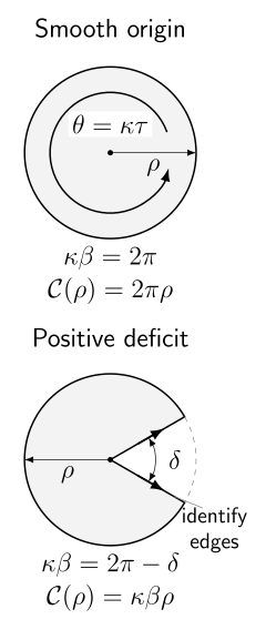
Smoothness requires $\mathcal C(\rho)/\rho=\kappa\beta=2\pi$ near a nonextremal horizon. The lower panel illustrates a positive deficit $\delta=2\pi-\kappa\beta$; the two marked edges are identified. This is an intrinsic local schematic, not a three-dimensional embedding or an extremal-horizon argument.

Boundary time fixes the physical temperature

The coordinate period alone is not an invariant thermometer reading. At a static wall $r=R$, proper Euclidean time is $d\tau_B=C\sqrt{f(R)}\,d\tau$, so

$$\beta_B=C\sqrt{f(R)}\,\beta, \qquad T_B=\frac{T_{\mathrm H}}{C\sqrt{f(R)}}.$$

This is the Euclidean form of Tolman redshift. With $C=1$ it gives the usual redshift from an infinity-normalized clock. With $C=f(R)^{-1/2}$, the coordinate $t$ is already wall proper time and $T_{\mathrm H}=T_B$. Rescale the generator by $\chi\mapsto a\chi$. Then $\kappa\mapsto a\kappa$, its coordinate time and period scale oppositely, and the proper boundary period remains the physical datum. Thus one may normalize at infinity in an asymptotically flat problem, by a chosen conformal-boundary clock in AdS, or at a finite cavity wall, but may not compare temperatures obtained from different normalizations without conversion.

For a rotating saddle, regularity identifies Euclidean time together with an angular shift generated by the horizon combination $\chi=\partial_t+\Omega_{\mathrm H}\partial_\phi$. A charged ensemble also fixes an admissible Euclidean gauge holonomy. Those chemical-potential data are additional boundary conditions; the scalar formula $\beta=2\pi/\kappa$ remains the local radial regularity condition for the properly normalized $\chi$.

Thermal interpretation and approximation regime

Euclidean periodicity becomes temperature because thermal correlation functions obey the KMS condition under imaginary-time translation. A smooth real Euclidean black-hole saddle prepares a regular equilibrium state when the analytic continuation and boundary conditions exist. Regularity alone does not establish which saddle dominates the partition function, nor does it derive an Unruh state describing evaporation. The former requires on-shell action differences; the latter is not an equilibrium Euclidean state.

The calculation is the leading stationary saddle approximation. The curvature radius and horizon scale must exceed the ultraviolet cutoff, matter fields are assumed to have the regular short-distance form appropriate to the Euclidean state, and backreaction is either included in the stationary saddle or consistently neglected. One-loop determinants and higher-curvature terms are the first omitted contributions. They can shift the effective action but do not change the local demand that a smooth nonextremal plane have angular period $2\pi$. Dimensional analysis supplies a quick check: $\kappa$ has inverse-length units, so $\beta$ has length units and $T$ has energy units in the adopted $c=\hbar=k_{\mathrm B}=1$ convention.

Extremal and singular limits

For an extremal horizon, $f(r)$ has a double rather than simple zero. The horizon lies at infinite proper distance on the Euclidean section, so the geometry has no finite-distance polar origin whose smoothness fixes $\beta$. Taking the nonextremal limit yields a temperature tending to zero, but the exact extremal Euclidean topology does not independently enforce that limit. This is a sharp counterexample to the claim that every Euclidean horizon fixes its temperature by removing a cone.

Likewise, a proposed complex metric need not possess a real polar plane, and a time-dependent horizon need not admit a single Euclidean time circle. Analytic continuation, integration contour, and state selection must then be supplied separately.

Exercise

For Schwarzschild in the asymptotic normalization $C=1$, $f(r)=1-2GM/r$ and $r_h=2GM$. Derive the smooth Euclidean period and the proper temperature at a cavity wall $R\gt2GM$. Show explicitly that the wall temperature approaches the Hawking temperature as $R\to\infty$.

Solution

At the horizon,

$$f'(r_h)=\frac{2GM}{r_h^2}=\frac{1}{2GM}, \qquad \kappa=\frac{f'(r_h)}{2}=\frac{1}{4GM}.$$

Therefore

$$\beta=\frac{2\pi}{\kappa}=8\pi GM, \qquad T_{\mathrm H}=\frac{1}{8\pi GM}.$$

The wall measures

$$T_B =\frac{1}{8\pi GM\sqrt{1-2GM/R}}.$$

As $R\to\infty$, the redshift factor tends to one and $T_B\to T_{\mathrm H}$. As the wall approaches the horizon, the local temperature diverges even though the generator-normalized temperature at infinity stays finite; this is a redshift effect, not a new surface gravity.

References

• Gibbons, G. W., and S. W. Hawking (1977), “Action Integrals and Partition Functions in Quantum Gravity,” Physical Review D 15, 2752–2756. DOI.
• Wald, R. M. (2001), “The Thermodynamics of Black Holes,” Living Reviews in Relativity 4, 6. Open PDF.