Mode Coupling and Broken Separability

Separability can fail in three different senses: the bulk differential operator may lack a commuting symmetry, a separable bulk operator may be paired with a nonseparable boundary, or nonlinear sources may couple modes even though the linear operator still separates. These cases demand different remedies. A controlled quadrupolar deformation makes the distinction explicit: its scalar wave operator couples only equal-$m$, equal-parity channels with $\Delta\ell=0,\pm2$ at first order. That sparse system can be reduced perturbatively in a nondegenerate regime, but this does not restore an exact Carter symmetry or justify an uncontrolled one-mode approximation.

Required background. Killing Fields and Isometry Groups supplies the distinction between manifest and hidden symmetries; Events, Intervals, and Minkowski Geometry supplies local field and frequency conventions.

Helpful background. Black-Hole Geometry and Mechanics fixes the undeformed horizon geometry; PDEs and Green Functions for Gravitation supplies coupled boundary-value problems and error norms; Formulations of General Relativity distinguishes a model metric from a solution of specified field equations; Frames, Coframes, and Anholonomy supplies the frame dependence of higher-spin components.

A quadrupolar scalar-wave model

Let $\mu=GM$, $f=1-2\mu/r$, and introduce the static, axisymmetric metric used as a controlled scalar-wave model by Ghosh, Franchini, Völkel, and Barausse:

$$\begin{aligned} g_{tt}&=-f\left[1+\varepsilon f_1(r)P_2(\cos\theta)\right],\\ g_{rr}&=f^{-1}\left[1-\varepsilon f_1(r)P_2(\cos\theta)\right],\\ g_{\theta\theta}&=(\sin\theta)^{-2}g_{\phi\phi} =r^2\left[1-\varepsilon f_1(r)P_2(\cos\theta)\right],\\ f_1(r)&=2f(r)\left(\frac{\mu}{r}\right)^3 . \end{aligned}$$

It is Schwarzschild at $\varepsilon=0$, has the leading asymptotic signature of an anomalous quadrupole, and leaves the horizon at $r=2\mu$ regular to the order retained. It is not an additional stationary, asymptotically flat, regular vacuum-GR black hole: the no-hair hypotheses prohibit that interpretation. The metric is instead an explicit beyond-Kerr test geometry, defined only through $O(\varepsilon)$. These construction limits and the resulting scalar equation are stated in Ghosh et al. 2023, § III.B, pp. 4–5, Eqs. (28)–(34).

For a massless scalar, expand the wave operator itself:

$$\mathcal L_\varepsilon=\Box_{g(\varepsilon)} =\Box_{\mathrm{Sch}}+\varepsilon\,\delta\Box_2 +O(\varepsilon^2).$$

The determinant explains why this particular deformation is tractable. Write $q=f_1P_2$. Through first order,

$$\sqrt{-g}=r^2\sin\theta(1-\varepsilon q)+O(\varepsilon^2).$$

The products $\sqrt{-g}\,g^{rr}$, $\sqrt{-g}\,g^{\theta\theta}$, and $\sqrt{-g}\,g^{\phi\phi}$ have no first-order correction, whereas $\sqrt{-g}\,g^{tt}=-r^2\sin\theta(1-2\varepsilon q)/f+O(\varepsilon^2)$. Substitution in the divergence formula for the scalar wave operator gives the off-shell identity

$$\delta\Box_2=q\Box_{\mathrm{Sch}}+\frac{2q}{f}\partial_t^2.$$

The first term cannot simply be omitted from the operator. Instead multiply the homogeneous equation by $1-\varepsilon q$, an invertible factor in the small-deformation regime, and then impose $e^{-i\omega t}$:

$$(\Box_{\mathrm{Sch}}-\varepsilon\mathcal J)\Psi =O(\varepsilon^2), \qquad \mathcal J[\Psi]=\frac{4\mu^3\omega^2}{r^3}P_2(\cos\theta)\Psi .$$

The multiplication term thus enters the reduced equation with a minus sign. For an inhomogeneous equation its source must be multiplied by the same factor. Every term in $\mathcal J$ has the dimensions of an inverse length squared, as does $\Box_{\mathrm{Sch}}$.

This reduced operator produces the coupling. Other metric deformations can also modify radial or angular derivatives; their coupling rules must be derived from their own $\delta\mathcal L$, not copied from this example.

Projection gives an exact first-order coupling rule

Expand $\Psi=e^{-i\omega t}r^{-1}\sum_{\ell m}Z_{\ell m}(r)Y_{\ell m}$ in the Condon–Shortley basis. Define

$$Q_{\ell m}=\sqrt{\frac{\ell^2-m^2}{4\ell^2-1}}, \qquad \ell\ge |m|,\quad \ell\ge1,$$

with $Q_{00}=0$ and every nonexistent harmonic or downward channel set to zero. In particular $Q_{|m|,m}=0$. Then

$$\cos\theta\,Y_{\ell m} =Q_{\ell+1,m}Y_{\ell+1,m}+Q_{\ell m}Y_{\ell-1,m}.$$

Applying this relation twice gives the complete product, not just a qualitative selection rule:

$$\begin{aligned} P_2(\cos\theta)Y_{\ell m} ={}&\frac32Q_{\ell+1,m}Q_{\ell+2,m}Y_{\ell+2,m}\\ &+\left[\frac32\left(Q_{\ell+1,m}^2+Q_{\ell m}^2\right)-\frac12\right] Y_{\ell m}\\ &+\frac32Q_{\ell m}Q_{\ell-1,m}Y_{\ell-2,m}. \end{aligned}$$

Axisymmetry preserves $m$, and even $P_2$ preserves parity; consequently only $\ell$, $\ell+2$, and $\ell-2$ occur. After the diagonal contribution is absorbed into $V_{\ell m}$, the model’s radial equations are

$$\frac{d^2Z_{\ell m}}{dr_*^2}+V_{\ell m}Z_{\ell m} =3\varepsilon\omega^2 f_1(r) \left(B_{\ell+2,m}Z_{\ell+2,m}+B_{\ell m}Z_{\ell-2,m}\right),$$

where $dr_*/dr=f^{-1}$, $B_{\ell m}=Q_{\ell-1,m}Q_{\ell m}$ for an existing downward channel, and

$$\begin{aligned} V_{\ell m} ={}&\omega^2-f\left[\frac{\ell(\ell+1)}{r^2} +\frac{2\mu}{r^3}\right]\\ &-\varepsilon f_1\omega^2 \left[3\left(Q_{\ell+1,m}^2+Q_{\ell m}^2\right)-1\right]. \end{aligned}$$

The undeformed limit is the massless scalar Schwarzschild equation. Moving the off-diagonal multiplication terms to the right explains their positive sign. These are Ghosh et al. 2023, § III.B, p. 5, Eqs. (30)–(34); they are exact for the first-order truncated equation, not for an unspecified all-orders metric.

More generally the coefficient of $Y_{\ell'm'}$ in $Y_{LM}Y_{\ell m}$ is $\int Y_{\ell'm'}^*Y_{LM}Y_{\ell m}\,d\Omega$. It vanishes unless

$$m'=m+M,\qquad |\ell-\ell'|\le L\le\ell+\ell', \qquad \ell+\ell'+L\ \text{is even}.$$

Valid magnetic indices are also required. Multiplication by $P_L$ is the $M=0$ case. These are necessary selection rules; the actual Gaunt coefficient still decides whether an allowed channel vanishes. The lower as well as upper triangle bound matters: $P_2Y_{00}$ has no monopole part.

Perturbative reduction is not exact separability

Two statements that can sound contradictory are both correct. The projected equations are coupled in the original spherical variables. Yet, for the specific $O(\varepsilon)$ system above, a near-identity radial field redefinition can remove off-diagonal terms when the relevant unperturbed channels are nondegenerate. Ghosh et al. construct such a reduction and check its quasinormal frequencies against the coupled system in Ghosh et al. 2023, § II, pp. 2–4 and § III.B, p. 5.

The elementary finite-dimensional analogue explains part of the regime. Suppose first that $L_0$ is Hermitian, its $u_j$ form an orthonormal basis, and $\lambda_\ell$ is simple. With $L=L_0+\varepsilon V$ and the correction chosen orthogonal to $u_\ell$, its eigenvector has the expansion

$$u_\ell(\varepsilon)=u_\ell +\varepsilon\sum_{j\ne\ell} \frac{\langle u_j,Vu_\ell\rangle}{\lambda_\ell-\lambda_j}u_j +O(\varepsilon^2).$$

A small denominator amplifies mixing. For a diagonalizable nonnormal matrix, replace the numerator by $w_j^\dagger Vu_\ell$, where $w_j^\dagger u_k=\delta_{jk}$, and choose the correction by $w_\ell^\dagger\delta u_\ell=0$ rather than Euclidean orthogonality. The norms of these dual vectors can be large even at a fixed eigenvalue gap. For example, in a fixed Euclidean norm,

$$L_\varepsilon= \begin{pmatrix}0&N\\ \varepsilon&1\end{pmatrix}, \qquad \lambda_\pm=\frac{1\pm\sqrt{1+4N\varepsilon}}2 .$$

The undeformed gap is one for every positive $N$, and the perturbing matrix has norm $|\varepsilon|$, yet the expansion parameter is $N\varepsilon$. A gap alone is not a perturbation bound. The pseudospectrum discussion develops the norm and conditioning issue.

A quasinormal problem is more generally a frequency-dependent operator equation $F(\omega,\varepsilon)u=0$, with outgoing and ingoing domain conditions; it is not automatically the matrix problem $Lu=\lambda u$. Order-by-order elimination requires a bounded inverse on the complementary channels, a controlled remainder, and a field transformation that preserves those boundary conditions. Near a multiple resonance one retains the resonant block rather than dividing by its small denominators.

Exact separability is stronger. It requires a product ansatz for the full operator and boundary problem, normally backed by commuting symmetry operators. The field-operator page proves the Kerr scalar commutator and exhibits a separate boundary-domain obstruction; see also Frolov, Krtouš, and Kubizňák 2017, § 6.3, pp. 119–120. An $O(\varepsilon)$ field redefinition says nothing about $O(\varepsilon^2)$, an order-one deformation, or a new Carter operator. Calling the reduced first-order equation “separable” is acceptable only when the perturbative qualifier and error order remain visible.

When coupled modes are necessary

A coupled angular-radial calculation is required whenever the requested accuracy resolves the discarded remainder or the reduction hypotheses fail. Near an avoided crossing or a degeneracy, the mixing denominator is comparable to $\varepsilon V_{\ell\ell'}$ and degenerate perturbation theory must retain the resonant block. A deformation with many angular multipoles produces a wide or dense coupling graph. Dynamical matter adds independent field channels rather than a prescribed potential, and eliminating them can create frequency-dependent nonlocal operators. None of these cases is captured by a single shifted radial potential without further proof.

Boundaries supply a separate obstruction. The bulk Schwarzschild wave operator still separates inside a surface $r=R_0[1+\varepsilon P_2(\cos\theta)]$, with $R_0\gt2\mu$ and a sufficiently small deformation to remain outside the horizon. Imposing Dirichlet data there gives, for a smooth field evaluated on the reference sphere,

$$\Phi(R_0,\theta,\phi) +\varepsilon R_0P_2(\cos\theta) \partial_r\Phi(R_0,\theta,\phi)=O(\varepsilon^2).$$

The same $\Delta\ell=0,\pm2$ rule now couples the boundary traces. The bulk commutator has not failed; the usual spherical boundary decomposition has. This is not a no-go theorem for separation in every possible coordinate system. Conversely, at second perturbative order on an exactly separable background, a quadratic source couples pairs of first-order modes through Gaunt coefficients while the linear operator acting on the second-order field remains separable. Source coupling is therefore not synonymous with broken linear separability.

A reproducible coupled-mode versus direct comparison

The coefficient rule predicts which channels occur, but not how many are enough for a chosen accuracy. To measure that second question, solve the same first-order equation in two angular representations, holding the source, frequency, radial domain, and boundary data fixed.

Fix the equation and the error norm

Use dimensionless $R=r/\mu$, $\Omega=\mu\omega$, $x=\cos\theta$, and the radially rescaled field $u=R\Phi$ after removing the time factor. Set $m=0$, $f=1-2/R$, and $f_1=2f/R^3$. Multiplying the reduced scalar equation by $Rf$ gives the following deliberately forced benchmark:

$$\begin{aligned} F_{\Omega,\varepsilon}u ={}&f^2\partial_R^2u+f(\partial_Rf)\partial_Ru +\frac f{R^2}\partial_x\!\left[(1-x^2)\partial_xu\right]\\ &+\left[\Omega^2-\frac{2f}{R^3} -2\varepsilon\Omega^2f_1P_2(x)\right]u =s(R)\chi_0(x). \end{aligned}$$

Here $R\in[2.5,10]$, $u=0$ at both radial walls, the poles are regular, and

$$\chi_\ell(x)=\sqrt{\frac{2\ell+1}{2}}P_\ell(x), \qquad s(R)=16\tau^2(1-\tau)^2, \qquad \tau=\frac{R-2.5}{7.5}.$$

Thus $\int_{-1}^{1}\chi_\ell\chi_j\,dx=\delta_{\ell j}$ and $Y_{\ell0}=\chi_\ell/\sqrt{2\pi}$. The source is a pure monopole. The finite inner wall is not a black-hole horizon, and the outer wall is not outgoing infinity. This is a frequency-domain boundary-value problem, not a quasinormal-mode or time-evolution calculation. Restoring dimensions means $r=\mu R$ and $\omega=\Omega/\mu$; the physical scalar operator carries an overall $\mu^{-2}$, while the prescribed benchmark source has the dimensionless normalization just stated.

Compare reconstructed fields using the fixed norm

$$\|u\|_w^2=\int_{2.5}^{10}\!\int_{-1}^{1} |u|^2\,\frac{dx\,dR}{f}, \qquad E_{\ell_{\max}}= \frac{\|u_{\ell_{\max}}-u_{\mathrm{2D}}\|_w} {\|u_{\mathrm{2D}}\|_w}.$$

The same norm can be written $\int|\Phi|^2R^2\,dx\,dR/f$; it is a chosen weighted $L^2$ norm, not a physical energy. For the residual $\rho=s\chi_0-F_{\Omega,\varepsilon}\widetilde u$, a bounded inverse would give

$$u-\widetilde u=F_{\Omega,\varepsilon}^{-1}\rho, \qquad \|u-\widetilde u\|_w \le\|F_{\Omega,\varepsilon}^{-1}\|_{w\to w}\,\|\rho\|_w.$$

A small omitted-forcing norm alone is therefore not an error certificate. The calculation below measures field differences directly. Its finite-matrix condition estimates are diagnostics, not bounds for this continuum inverse.

Independent angular representations

The coupled calculation retains even Legendre modes through $\ell_{\max}$ and projects $P_2$ using the exact coefficients above. The direct calculation uses Chebyshev–Lobatto nodes in $x$, differentiates $\partial_x[(1-x^2)\partial_xu]$ as a differential operator, and multiplies by $P_2(x)$ pointwise. It does not use the harmonic coupling matrix. At the poles the regular angular operator becomes $-2x\partial_xu$; no extra polar Dirichlet condition is added.

Both methods use radial Chebyshev collocation, so radial refinement is an additional required check, not an independent second radial method. The reference has radial degree 64 and angular degree 20. Separate sweeps vary radial degree through 40, 48, and 56 and angular degree through 10, 14, and 18; joint 80/24 refinements test both frequencies at $\varepsilon=0,2$. Independent Gauss quadrature evaluates norms, checks the coupling matrix, and compares the full off-grid PDE residual with the omitted angular forcing. A polynomial manufactured solution with $\ell=0,2,4$ checks derivative signs, coefficients, and both implementations.

The complete comparison uses $\varepsilon=0,0.25,0.5,1,2$, $\ell_{\max}=0,2,4,6,8$, and $\Omega=0.35-0.025i,\ 0.55-0.01i$. The high-$\varepsilon$ cases stress the fixed first-order PDE. Even though the largest retained metric fraction at $\varepsilon=2$ is only $27/512\simeq0.0527$, this gives no bound on the unknown second-order metric coefficients. Numerical convergence cannot certify that omitted physics.

The figure shows how truncation error changes with channel count at the second frequency. Inspect both the decrease along each curve and the larger errors at larger deformation. Results reaching the comparison floor are unresolved there, not exact agreement.

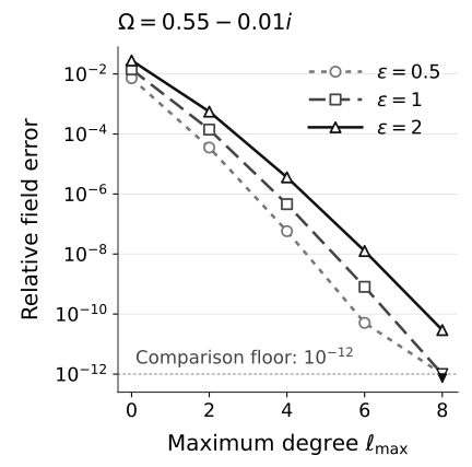
Quantitative truncation comparison for the first-order scalar equation at $\Omega=0.55-0.01i$, $R\in[2.5,10]$, regular poles, zero radial Dirichlet walls, and the pure-monopole source above. Relative error uses $\|u\|_w^2=\int|u|^2\,dx\,dR/f$ against direct two-dimensional collocation. Markers and line styles distinguish $\varepsilon=0.5,1,2$; values below $10^{-12}$ are unresolved at the empirical comparison floor. This is not a quasinormal-spectrum error or an all-orders metric error.

At the largest tested deformation, the two frequencies give:

$\ell_{\max}$	$E_{\ell_{\max}}$, $\Omega=0.35-0.025i$	$E_{\ell_{\max}}$, $\Omega=0.55-0.01i$
0	$2.606\times10^{-2}$	$2.810\times10^{-2}$
2	$1.166\times10^{-4}$	$5.554\times10^{-4}$
4	$2.438\times10^{-7}$	$3.600\times10^{-6}$
6	$3.136\times10^{-10}$	$1.261\times10^{-8}$
8	Below the $10^{-12}$ comparison floor	$2.930\times10^{-11}$

The largest joint reference-refinement difference is $4.53\times10^{-13}$; both manufactured-solution errors are below $3\times10^{-14}$. These checks support the reported comparison floor empirically, not as a rigorous continuum bound. For example, $\ell_{\max}=4$ misses a $10^{-6}$ relative field target at the second frequency and $\varepsilon=2$, while $\ell_{\max}=6$ meets it in this benchmark. A different source, domain, or frequency requires a new test.

Download the Python calculation, pinned requirements, and complete results. The saved run used CPython 3.9.6. In an isolated environment with those files together, run:

python3 -m pip install -r quadrupole-coupling-requirements.txt
python3 quadrupole-coupling.py --verify-saved quadrupole-coupling-results.json

The program recomputes all 50 comparisons and every saved convergence and residual record, failing if a required check or saved-result comparison fails. The results record the source fingerprint and runtime versions. The Python version and timing are retained as provenance, not required to match; unresolved floating-point digits are also excluded from exact comparison.

Separation and coupling results through 2026-09-05

The evidence and literature status below are assessed through 2026-09-05. They support regime-dependent decisions, not a universal claim that small deformations either always decouple or always require a two-dimensional solver.

Formulation	Coupling structure	What is established	What remains uncontrolled
Exact Kerr scalar equation	Spheroidal basis at fixed $m$	Full radial–angular separation follows from the Carter structure	Completeness under quasinormal boundary conditions is a separate question
Specified non-Kerr separable families	Special radial metric functions within a named axisymmetric ansatz	Both massive scalar and Hamilton–Jacobi equations separate	Not a classification of every axisymmetric metric or field equation
Static anomalous-quadrupole model at $O(\varepsilon)$	Same $m$ and parity; $\Delta\ell=0,\pm2$	Coupled and perturbatively reduced quasinormal calculations agree in the tested regime	The metric and equation omit $O(\varepsilon^2)$, and the published check is not a direct two-dimensional evolution
This page’s forced annulus comparison	Same first-order quadrupole, five deformations and five angular truncations	Weighted field differences agree under independent angular and radial refinement; explicit errors above	Fixed complex frequencies and radial walls, not quasinormal conditions or direct time evolution
Prescribed $W(r)P_L(\cos\theta)$ potential	Finite Wigner band with $\lvert\ell-\ell'\rvert\le L$	Projection coefficients are exact once $W$ and $L$ are named	A corrected hidden symmetry or all-order decoupling is not generic
Deformed surface $r=R(\theta)$	Boundary traces couple even if the bulk separates	Taylor projection gives a controlled sparse boundary system for small deformation	Large deformations and corner or low-regularity boundaries need direct multidimensional treatment
Quadratic perturbative source	Triangle and spin-weight selection rules	Each sourced mode can be evolved with the background’s separated Green function	Strong backreaction and resummation beyond the perturbative data class remain open

Non-Kerr separability is not wholly undiscovered: Konoplya, Stuchlík, and Zhidenko 2018, §§ II.A–II.C, p. 5, Eqs. (22)–(30) exhibit a family with freely specified radial functions within their metric ansatz. Their result does not make an arbitrary deformation separable.

The quadrupole paper reports that truncations at $\ell_{\max}=\ell+2$ and $\ell+4$ differed by less than the linear-in-$\varepsilon$ approximation error in the cases tested. Its comparison is between coupled-mode and perturbatively reduced quasinormal calculations, not direct two-dimensional time evolution Ghosh et al. 2023, § III.B, p. 5.

A separate 2026 preprint demonstrates a two-dimensional frequency-domain neural-network calculation of Kerr gravitational modes without a radial–angular product ansatz. It tests six branches through spin $a/\mu=0.9998$ against independent Leaver-based frequencies, reporting each frequency-component error below $0.5\%$; beyond-Kerr applications remain prospective Ferrer-Sánchez et al. 2026, § IV, p. 10 and § V, p. 18. This is a method benchmark on a separable background, not evidence that the quadrupolar non-Kerr spectrum has been computed to that accuracy.

Sparse perturbative mixing can be removed or truncated efficiently when the complementary response and the small-$|\varepsilon|$ remainder are controlled. On the other hand, near-degenerate spectra, continuum coupling, incompatible boundaries, or order-one deformation can make the genuinely coupled formulation indispensable. For a specified new family one must still test its operator and boundary problem; known separable examples do not settle that family-specific question. A rigorous truncation bound could establish control; comparison with a direct two-dimensional solution could demonstrate breakdown. A newly identified symmetry or a correction to the coupling coefficients could change the conclusion.

General representation theory remains mathematical preparation, while the classification and parent geometry of hidden symmetries remain in Exact Spacetimes. The present scope is the harmonic diagnostic that decides what a specified black-hole perturbation operator and its boundary conditions actually couple.

Exercise: determine the first omitted quadrupole channel

Start from the normalized monopole $Y_{00}$. Use the $Q_{\ell m}$ formula to show that $P_2Y_{00}=Y_{20}/\sqrt5$. If the field is seeded only in $\ell=0$, which channels are required through first order in $\varepsilon$, and which new channel first appears at second order? State the assumption behind this power counting.

Solution

For $(\ell,m)=(0,0)$,

$$Q_{10}=\frac1{\sqrt3}, \qquad Q_{20}=\frac2{\sqrt{15}}.$$

The upward coefficient in the product formula is

$$\frac32Q_{10}Q_{20} =\frac32\frac1{\sqrt3}\frac2{\sqrt{15}} =\frac1{\sqrt5}.$$

The diagonal coefficient is $\tfrac32Q_{10}^2-\tfrac12=0$, and no negative-$\ell$ harmonic exists. Hence $P_2Y_{00}=Y_{20}/\sqrt5$, consistent with $P_2=\sqrt{4\pi/5}\,Y_{20}$ and $Y_{00}=1/\sqrt{4\pi}$.

The $\ell=0$ seed sources $\ell=2$ at $O(\varepsilon)$, so a first-order reconstruction retains $\ell=0,2$. Acting once more on the induced quadrupole produces $\ell=4$ at $O(\varepsilon^2)$, as well as corrections to $\ell=0,2$. This ordering assumes a regular perturbation expansion with bounded complementary-channel inverses in a specified norm, not merely separated eigenvalues. Near a degeneracy, the nominal $O(\varepsilon)$ response can be enhanced and the simple channel-counting estimate is not a valid error bound.

Exercise: a small residual without a nearby eigenvalue

For the displayed nonnormal matrix take $N=100$, $\varepsilon=1/100$, the unit vector $v=(1,0)^T$, and trial eigenvalue zero. Compute the residual norm and the distance to the nearest exact eigenvalue. Why do these numbers not contradict the residual identity for an invertible operator?

Solution

The residual is $L_\varepsilon v=(0,1/100)^T$, with Euclidean norm $0.01$. The eigenvalues are $(1\pm\sqrt5)/2$, so the nearest one is a distance $(\sqrt5-1)/2\simeq0.618$ from zero. The familiar Hermitian bound of spectral distance by residual norm does not apply to this nonnormal matrix. An inverse-norm bound remains true, but its amplification factor need not be small. Thus a numerically small discarded forcing or eigenvalue residual must not be reported as an equally small field or spectral error without the corresponding conditioning information.

References

• Ferrer-Sánchez, Antonio, Daniela D. Doneva, José D. Martín-Guerrero, Stoytcho S. Yazadjiev, Roberto Ruiz de Austri-Bazan, Yolanda Vives-Gilabert, and José A. Font. “Kerr Quasinormal Modes without Variable Separation: A Two-Dimensional Hyperboloidal Teukolsky Solver with Physics-Informed Neural Networks.” Preprint (2026). arXiv:2608.19774.
• Frolov, Valeri P., Pavel Krtouš, and David Kubizňák. “Black Holes, Hidden Symmetries, and Complete Integrability.” Living Reviews in Relativity 20 (2017): 6. arXiv.
• Ghosh, Rajes, Nicola Franchini, Sebastian H. Völkel, and Enrico Barausse. “Quasi-Normal Modes of Non-Separable Perturbation Equations: The Scalar Non-Kerr Case.” Physical Review D 108 (2023): 024038. DOI, arXiv.
• Konoplya, R. A., Z. Stuchlík, and A. Zhidenko. “Axisymmetric Black Holes Allowing for Separation of Variables in the Klein-Gordon and Hamilton-Jacobi Equations.” Physical Review D 97 (2018): 084044. DOI, arXiv.