Pseudospectra and Nonnormal Sensitivity

A pseudospectrum measures the size of a linear evolution’s frequency-domain response, including frequencies away from resonance. For a black hole, however, there is no meaningful “the pseudospectrum” until the evolution generator, its domain, the endpoint conditions, and the norm have all been fixed. Resolvent amplification beyond the normal-operator benchmark diagnoses nonnormality in that realization. Contour width alone does not: it also depends on the spectrum and the chosen contour level. Nor does it, by itself, establish growing energy, an astrophysically reachable environmental change, or an observable detector signal.

Required background. PDEs and Green Functions for Gravitation supplies closed operators, resolvents, domains, and evolution estimates.

Helpful background. Black-Hole Geometry and Mechanics supplies the horizon and null-infinity geometry; Formulations of General Relativity supplies perturbative variables; Computational Relativity supplies spectral convergence; Black-Hole Perturbation Theory supplies the master equations. Within this chapter, Quasinormal Boundary Conditions and Resonances fixes the resonance problem and Spectral Collocation and Direct Eigenvalue Methods develops its numerical realization.

Why nonnormality changes the question

For a matrix $B$ and a chosen inner product, normality means

$$BB^\dagger=B^\dagger B.$$

A normal matrix has an orthonormal eigenbasis. If all of its time-generator eigenvalues lie in the left half-plane, every modal component decays and no cancellation between almost parallel eigenvectors can hide a later burst. A nonnormal matrix need not have orthogonal eigenvectors. Large coefficients can cancel at one time and fail to cancel later, so eigenvalues alone no longer determine the largest forced response or transient.

The dagger is part of the physics: it depends on the inner product. Changing the energy or regularity norm changes the adjoint, the operator norm, the resolvent norm, and therefore the pseudospectrum. It does not change the algebraic eigenvalues of a finite matrix under a similarity transformation.

The reference against which “large” must be judged is precise. For a normal matrix, or a closed normal operator on a Hilbert space, the spectral theorem gives

$$\lVert(zI-B)^{-1}\rVert =\frac{1}{\operatorname{dist}(z,\sigma(B))}, \qquad z\notin\sigma(B).$$

Thus a normal operator’s $\varepsilon$-pseudospectrum is just the open $\varepsilon$-neighborhood of its spectrum. Many nearby eigenvalues, or a large $\varepsilon$, can make this set broad without any nonnormality. A resolvent strictly larger than the displayed benchmark rules out normality in that same Hilbert norm; equality at one sampled point does not prove normality.

Schwarzschild evolution, energy, and domain

A concrete hyperboloidal equation

Fix the four-dimensional Schwarzschild exterior and its axial Regge–Wheeler field with $\ell=2$. Set $T_0=4GM$ and use dimensionless time and frequency in this section: a mode $e^{-i\omega\tau}$ has physical frequency $\omega/T_0$. The minimal-gauge coordinates are

$$\begin{aligned} \sigma&=\frac{2GM}{r},& \frac{t}{T_0}&=\tau-h(\sigma),& \frac{r_*}{T_0}&=g(\sigma),\\ h(\sigma)&=\frac12\left[\ln\sigma+\ln(1-\sigma)-\frac1\sigma\right],\\ g(\sigma)&=\frac12\left[\frac1\sigma+\ln(1-\sigma)-\ln\sigma\right]. \end{aligned}$$

Here $0\lt\sigma\lt1$ covers the exterior, with future null infinity at $\sigma=0$ and the future horizon at $\sigma=1$. Unlike the tortoise coordinate, $\sigma$ increases toward the hole. Define $\psi=\partial_\tau\phi$ and $u=(\phi,\psi)^T$. The regular differential expression is

$$\begin{aligned} \partial_\tau u&=A_0u,\\ A_0\begin{pmatrix}\phi\\ \psi\end{pmatrix} &=\begin{pmatrix} \psi\\[3pt] \displaystyle\frac{\partial_\sigma(p\,\partial_\sigma\phi)-q\phi +2\gamma\,\partial_\sigma\psi+\gamma'\psi}{w} \end{pmatrix},\\ w&=2(1+\sigma),&p&=2\sigma^2(1-\sigma),\\ q&=12-6\sigma,&\gamma&=1-2\sigma^2. \end{aligned}$$

A prime denotes $d/d\sigma$. These coefficients follow by transforming the Regge–Wheeler wave equation, not by imposing reflecting endpoint rows: $p=-1/g'$, $\gamma=ph'$, $w=(1-\gamma^2)/p$, and $q=T_0^2V_{\rm RW}/p$. This also fixes the time scale of the comparison Jaramillo–Panosso Macedo–Al Sheikh 2021, §VI.A, eqs. (69)–(73), p. 031003-23.

For a specified evolution realization $A$, set $L=iA$. In the site’s Fourier convention,

$$i\partial_\tau u=L u, \qquad u=(\phi,\psi)^T, \qquad u(\tau)=e^{-i\omega\tau}u_\omega.$$

Thus $Lu_\omega=\omega u_\omega$ for an eigenvector in its domain, and decay means $\operatorname{Im}\omega\lt0$. The source instead writes $\partial_\tau u=iL_{\rm JMA}u$ with modes $e^{+i\omega_{\rm JMA}\tau}$. At the same time scale, the complete translation is

$$L=-L_{\rm JMA}, \qquad \omega=-\omega_{\rm JMA}.$$

What the energy identity proves

The positive energy product, up to a fixed overall physical normalization, is

$$\langle u_1,u_2\rangle_E =\frac12\int_0^1 \left[ w\,\bar\psi_1\psi_2 +p\,\partial_\sigma\bar\phi_1\partial_\sigma\phi_2 +q\,\bar\phi_1\phi_2 \right]d\sigma.$$

Let $E(\tau)=\lVert u(\tau)\rVert_E^2$. For a smooth solution, substitute the second evolution equation into $dE/d\tau$. Integration by parts cancels the bulk $\phi$–$\psi$ terms. The remaining transport terms are also a total derivative,

$$2\gamma\operatorname{Re}(\bar\psi\psi')+\gamma'|\psi|^2 =(\gamma|\psi|^2)',$$

giving

$$\begin{aligned} \frac{dE}{d\tau} &=\left[\operatorname{Re}(p\bar\psi\,\partial_\sigma\phi) +\gamma|\psi|^2\right]_0^1\\ &=-|\psi(0)|^2-|\psi(1)|^2\leq0. \end{aligned}$$

The last equality uses $p(0)=p(1)=0$, $\gamma(0)=1$, and $\gamma(1)=-1$. Both endpoints remove energy. Dissipation does not itself prove nonnormality: the normal scalar evolution $\dot u=-u$ also dissipates. Nor can nonnormality reverse this energy inequality. A component or an extraction observable may grow while this total energy decreases.

Closed generators and their domains

The coefficients above do not, alone, define a continuum spectrum. Let $H_E$ be the completion of smooth pairs on $[0,1]$ in this energy norm, and initially let $A_0$ act on those smooth pairs. It is densely defined and closable: if $u_n\to0$ and $A_0u_n\to v$ in $H_E$, both convergences hold in local distributions; the differential expression then gives $v=0$. Its graph closure is consequently a closed dissipative operator. Without this single-valued-closure argument, simply writing down a graph norm would not prove closedness.

Identifying that closure with a retarded evolution generator requires more, such as maximal dissipativity or an independently established well-posed evolution. Dissipativity alone is insufficient. If $T(\tau)$ is the chosen strongly continuous retarded semigroup on $H_E$, its generator domain is precisely

$$D(A)=\left\{u\in H_E: \lim_{\tau\downarrow0}\frac{T(\tau)u-u}{\tau} \text{ exists in }H_E\right\}.$$

The limit defines $Au$, and this generator is closed. The energy inequality passes to a continuous extension of the smooth retarded evolution by density, giving $\lVert T(\tau)\rVert_E\leq1$. Pointwise endpoint traces of arbitrary graph-domain states require additional justification; only the smooth-core flux equality was derived above. This page does not prove the requisite existence theorem, a core theorem for $A_0$, or equality between the energy-space spectrum and the isolated continued QNM poles. Subsequent continuum resolvent statements concern a fixed closed realization with the stated hypotheses, not an unspecified differential expression.

The distinction matters at null infinity, where $p$ has a double zero. Bounded endpoint solutions need not be QNMs, and even the word “regular” is insufficient without a function class and the retarded continuation prescription. The modern hyperboloidal formulation treats this regularity issue explicitly Macedo–Zenginoğlu 2025, §3.3, “From geometry to analysis”. Use the continued retarded branches when identifying resonances; do not impose smoothness anew at an exceptional frequency.

For a different regularity question, one may instead complete smooth data in a declared Sobolev family, for integer $k\geq0$,

$$\lVert u\rVert_{H_E^k}^2 =\sum_{j=0}^{k}\left\lVert\partial_\sigma^j u\right\rVert_E^2.$$

Larger $k$ penalizes fine spatial structure. The Hilbert space and generator domain must be specified afresh; different continuum completions need not be related by a bounded invertible similarity. An $H_E^k$ contour cannot be relabeled as an energy contour after the calculation.

Resolvents, quasimodes, and perturbations

For a frequency $\omega$ outside the spectrum of the closed realization,

$$R_L(\omega)=(\omega I-L)^{-1}.$$

In one declared operator norm, define

$$\sigma_\varepsilon(L) =\left\{\omega:\lVert R_L(\omega)\rVert>\varepsilon^{-1}\right\} \cup\sigma(L).$$

For a finite matrix with unrestricted complex perturbations, this has two equivalent readings:

• $\omega\in\sigma_\varepsilon(L)$ if a perturbation $\delta L$ with $\lVert\delta L\rVert<\varepsilon$ can make $\omega$ an eigenvalue;
• $\omega\in\sigma_\varepsilon(L)$ if a unit vector $v$ satisfies $\lVert(L-\omega I)v\rVert<\varepsilon$, so $v$ is a quasimode.

For an unbounded operator, these equivalences require compatible closed-operator hypotheses and a declared perturbation class. A small bounded potential perturbation does not include changing the domain, moving null infinity to a reflecting wall, or altering the asymptotic spacetime. The matrix equivalences and their norm dependence are developed in Trefethen–Embree 2005, Chapters 2 and 4; the black-hole specialization is given in Jaramillo–Panosso Macedo–Al Sheikh 2021, §§III.B.1–III.B.4, pp. 031003-10–031003-11.

The usual pseudospectrum is unstructured: it allows every bounded perturbation of the stated operator norm, not just changes generated by an admissible matter distribution or potential. Restricting that class defines a structured sensitivity problem whose reachable spectral points can form a strict subset. An unstructured contour therefore bounds what a physical perturbation might do; it does not demonstrate that the physical class reaches the contour.

The logical ladder is therefore:

1. A large resolvent means that some normalized forcing is strongly amplified in the chosen input/output norm.
2. Under the stated matrix or closed-operator hypotheses, a pseudospectral point can describe an unstructured spectral perturbation or an accurate quasimode. Its distance from the spectrum must be compared with $\varepsilon$; reachability by a restricted physical class is a separate question.
3. Transient growth means $\lVert e^{-iL\tau}\rVert>1$ in the same state norm for some $\tau$.
4. A changed waveform additionally needs specified initial data or a source, propagation to an extraction observable, and non-negligible excitation.
5. A detector claim additionally needs a noise model, inference procedure, and a resolvable difference.

No step automatically supplies the next one.

When a resolvent bound does force growth

Let $A=-iL$ generate a strongly continuous semigroup $T(t)$ in the same norm, and suppose $M_*:=\sup_{t\geq0}\lVert T(t)\rVert$ is finite. For $\operatorname{Re}z\gt0$, the Laplace representation gives

$$\begin{aligned} (zI-A)^{-1}&=\int_0^\infty e^{-zt}T(t)\,dt,\\ \lVert(zI-A)^{-1}\rVert&\leq\frac{M_*}{\operatorname{Re}z},\\ M_*&\geq(\operatorname{Re}z)\lVert(zI-A)^{-1}\rVert. \end{aligned}$$

The last line is a resolvent lower bound on maximum transient amplification. If $M_*=\infty$, it is only a trivial lower bound; one must not use the bounded-semigroup integral without its convergence hypothesis. For a stable finite matrix the hypothesis holds. At a point inside its $\varepsilon$-pseudospectrum with positive real part, $M_*\gt\operatorname{Re}z/\varepsilon$. Thus $\operatorname{Re}z\gt\varepsilon$ is a sufficient contour-based test for growth above one. Merely crossing $\operatorname{Re}z=0$ is not.

For example, $A=-1$ is normal and $T(t)=e^{-t}$ is contractive, yet its $\varepsilon=2$ pseudospectrum, $|z+1|\lt2$, enters $\operatorname{Re}z\gt0$. A contractive semigroup permits this: its resolvent bound only confines the pseudospectrum to $\operatorname{Re}z\lt\varepsilon$ in the right half-plane. The lower bound says nothing about the maximizing time, the required initial state, or a detector response. These require separate calculations.

One linear map in two norms

It is easiest to see the distinction in the ordinary time-generator plane. Set

$$A=-iL, \qquad \partial_\tau u=A u, \qquad z=-i\omega.$$

The lower half of the black-hole frequency plane, $\operatorname{Im}\omega<0$, maps to the left half of the generator plane, $\operatorname{Re}z<0$. The figure below uses the $z$ plane; it is not a plot of black-hole frequencies.

Consider the exact finite map

$$A_K=\begin{pmatrix}-1&K\\0&-2\end{pmatrix}, \qquad (zI-A_K)^{-1} =\begin{pmatrix} \dfrac{1}{z+1}&\dfrac{K}{(z+1)(z+2)}\\[6pt] 0&\dfrac{1}{z+2} \end{pmatrix}.$$

Its eigenvalues remain $-1$ and $-2$ for every $K$, but the off-diagonal resolvent entry grows with $K$. For $K=20$, choose

$$S=\operatorname{diag}(20,1), \qquad \lVert u\rVert_S=\lVert S^{-1}u\rVert_2.$$

The induced operator norm obeys

$$\lVert B\rVert_S=\lVert S^{-1}BS\rVert_2, \qquad S^{-1}A_{20}S =\begin{pmatrix}-1&1\\0&-2\end{pmatrix}.$$

The same linear map and eigenvalues therefore have different resolvent norms. At $z=0$ the smallest singular values of the two matrix pencils are $0.0993820$ and $0.8740320$, respectively. In the Euclidean norm, $z=0$ already lies inside the $\varepsilon=0.10$ pseudospectrum; in the weighted norm it does not. This particular crossing is not yet a growth bound. Inspect the dashed stability boundary and the unchanged black eigenvalue markers in the quantitative comparison.

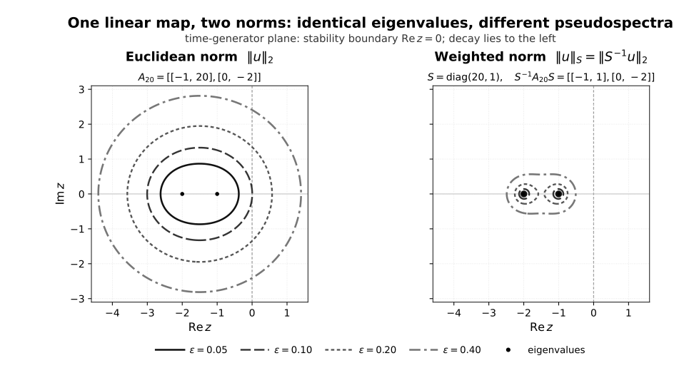
Quantitative finite-matrix comparison, not a black-hole spectrum. Each curve is the boundary $s_{\min}(zI-M)=\varepsilon$ for $\varepsilon=0.05,0.10,0.20,0.40$. The left panel uses $M=A_{20}$ in the Euclidean norm. The right uses $M=S^{-1}A_{20}S$ because $\lVert u\rVert_S=\lVert S^{-1}u\rVert_2$. Similarity preserves the eigenvalues $-1$ and $-2$ while the induced resolvent norm and pseudospectrum change: the Euclidean $\varepsilon=0.40$ contour reaches $\operatorname{Re}z\simeq1.4017$, whereas the weighted contour reaches only $\operatorname{Re}z\simeq-0.5122$. These are axes for $e^{tA_{20}}$, where stability means $\operatorname{Re}z<0$, not the $e^{-i\omega\tau}$ frequency plane, where decay means $\operatorname{Im}\omega<0$.

The same example separates spectral stability from transient growth. The resolvent at $z=1$ already certifies amplification in the Euclidean norm:

$$M_*\geq\lVert(I-A_{20})^{-1}\rVert_2 =\sqrt{\frac{413+\sqrt{170425}}{72}} \simeq3.38671.$$

This bound exceeds one but does not give the actual maximum. To find that maximum, use the exact propagator

$$e^{tA_K} =\begin{pmatrix} e^{-t}&K(e^{-t}-e^{-2t})\\ 0&e^{-2t} \end{pmatrix}.$$

For $K=20$, direct singular-value maximization gives

$$\lVert e^{0.5A_{20}}\rVert_2=4.82523, \qquad \max_{t\ge0}\lVert e^{tA_{20}}\rVert_2 =5.03137$$

at $t\simeq0.685619$. Both eigenvalues are still negative. In the weighted norm the Hermitian part of $S^{-1}A_{20}S$ has largest eigenvalue

$$\mu_2=\frac{-3+\sqrt2}{2}<0,$$

so $\lVert e^{tA_{20}}\rVert_S\le e^{\mu_2t}\le1$. The transient is real in one norm and absent in the other. This does not make either norm “wrong”; it shows that a physical claim must say which quantity is being measured.

The editable generator evaluates the $2\times2$ singular values analytically, checks them against direct LAPACK singular-value decompositions at independent complex points, checks the exact similarity transform and stability-boundary values, and verifies the transient maximum separately. It does not discretize a black-hole operator.

From a matrix plot to a black-hole computation

At numerical resolution $N$, let $L_N$ approximate $L$ and let $G_N=F_N^*F_N$ be the Gram matrix of the declared continuum scalar product. Then

$$\left\lVert(\omega I-L_N)^{-1}\right\rVert_{G_N} =\frac{1}{s_{\min}\!\left[F_N(\omega I-L_N)F_N^{-1}\right]}.$$

A smooth contour is not a convergence test. A credible continuum calculation must:

1. state the hyperboloidal chart, compactification, endpoint trace class, graph domain, norm, and spectral window;
2. verify $G_N>0$ and report the conditioning of its factorization;
3. compare both isolated poles and off-pole resolvent values at several resolutions;
4. repeat the operator construction with different residual conditions or endpoint discretization, not merely a denser version of the same matrix or a change of basis;
5. repeat in the energy norm and in each claimed $H_E^k$ norm;
6. identify nonconvergent eigenvalue strings used to approximate a branch cut without deleting their time-domain contribution;
7. perturb only within the declared continuum class and check that migrated eigenvalues remain inside the matching contour.

The Chebyshev and Gram-matrix construction used in the foundational Schwarzschild calculation is documented in Jaramillo–Panosso Macedo–Al Sheikh 2021, Appendices B–C, pp. 031003-35–031003-38. Agreement of a few QNM poles is insufficient: the poles can converge while an ill-conditioned resolvent does not.

Direct evolution provides an independent check. Compute

$$G(\tau)=\left\lVert e^{-iL\tau}\right\rVert$$

in the same norm, evolve a maximizing right singular vector and localized finite-energy data, and ask whether both the maximizing data and the growth curve survive refinement. For the dissipative Schwarzschild exterior, energy cannot increase, yet optimized sums of QNMs can produce increasingly long energy plateaus before modal decay. Carballo and Withers demonstrate this with axial $\ell=2$ Schwarzschild QNM sums Carballo–Withers 2024, arXiv v3, §5, pp. 25–27, Fig. 10. Their plotted energy ratio is a squared state norm; it must not be confused with the unsquared $G(\tau)$ defined here.

Three finite Schwarzschild approximations

The distinction between one waveform and a worst-case response can be tested on the Schwarzschild equation above. The downloadable computation compares three finite methods, each in the energy and $H_E^1$ norms. It retains every endpoint degree of freedom and every finite eigenvalue. No reflecting endpoint row or eigenvalue clipping is introduced. For each method and resolution, changing the norm leaves the finite evolution matrix unchanged.

Strong Chebyshev–Lobatto collocation imposes the differential equation at interpolation nodes. Weak shifted-Legendre Galerkin projection instead requires its residual to be orthogonal to the test space in the integrated equation. Both use global polynomials of degree at most $N$, but their different residual conditions give different matrices: they are not a single operator written in two bases. The third method uses weak $C^2$ quintic Hermite elements on a uniform mesh. This is a genuinely different, piecewise-polynomial trial space.

The polynomial degrees are $12,20,32,48,64,80$; the element counts are $4,6,10,16,24,32$. These correspond to state dimensions $2(N+1)$ and $6(m+1)$, respectively. The extra continuity in the element method is consequential: a jump in $\phi''$ could produce a jump in the acceleration and hence a distributional contribution to its derivative. An elementwise $H_E^1$ residual would miss that contribution. The $C^2$ construction and independent acceleration-trace checks avoid this particular defect; they do not prove continuum convergence. This does not disqualify $C^1$ elements from a weak energy formulation: the extra continuity serves this particular higher-derivative action test.

Weak projection preserves energy loss

For real trial functions $b_j$, let $\phi=\sum_j a_jb_j$ and $\psi=\sum_j v_jb_j$. Integrating the second evolution equation against $b_i$ gives

$$\begin{aligned} W_{ij}&=\int_0^1w b_i b_j\,d\sigma,\\ K_{ij}&=\int_0^1(p b_i'b_j'+q b_i b_j)\,d\sigma,\\ C_{ij}&=\int_0^1b_i(2\gamma b_j'+\gamma' b_j)\,d\sigma,\\ A_N&=\begin{pmatrix}0&I\\-W^{-1}K&W^{-1}C\end{pmatrix}, \qquad G_E=\frac12\begin{pmatrix}K&0\\0&W\end{pmatrix}. \end{aligned}$$

The boundary term from $p\phi'$ vanishes because $p$ vanishes at both endpoints. If $e_0$ and $e_1$ are the columns with entries $b_j(0)$ and $b_j(1)$, integration of $(2\gamma b_i b_j)'$ yields

$$\begin{aligned} C+C^T&=-2(e_0e_0^T+e_1e_1^T),\\ A_N^*G_E+G_EA_N &=-\begin{pmatrix}0&0\\0&e_0e_0^T+e_1e_1^T\end{pmatrix}\leq0. \end{aligned}$$

Thus both weak semidiscrete evolutions are contractive in this energy norm in exact arithmetic. This property follows from their construction, not from clipping an unwanted eigenvalue afterward. Strong collocation need not preserve the same integrated identity, even when the energy of its interpolating polynomial is evaluated accurately.

A fixed pulse versus the largest response

For a finite propagator $T_N(\tau)=e^{\tau A_N}$, one initial state measures only one direction. Here $X$ denotes either $E$ or $H_E^1$; the Gram factor is chosen for that norm:

$$r_X(\tau;u_{0,N}) =\frac{\lVert T_N(\tau)u_{0,N}\rVert_X}{\lVert u_{0,N}\rVert_X} \leq\lVert T_N(\tau)\rVert_X.$$

The operator norm maximizes over all nonzero initial states. Agreement for one pulse supplies no upper bound on that largest response. Use the same smooth datum, represented exactly in all three spaces:

$$\phi_0=0,\qquad\psi_0=\sigma(1-\sigma),\qquad \lVert u_0\rVert_E^2=\frac1{20},\qquad \lVert u_0\rVert_{H_E^1}^2=\frac{11}{20}.$$

At dimensionless time $\tau=8$, the largest tested configurations give the following energy-norm comparison. At fixed exterior radius, this is an elapsed Schwarzschild time of $32GM$.

Method and resolution	Operator norm	Fixed-pulse norm ratio
Collocation, $N=80$	2.21136	0.07000045
Weak Legendre, $N=80$	1.00000	0.07000045
Weak Hermite, $m=32$	1.00000	0.07000045

The weak values round to one; their exact finite energy identity guarantees at most one, not equality.

These are unsquared state-norm ratios, not energy ratios. The pulse’s remaining energy fraction is approximately $0.00490006$, the square of its norm ratio. The reported pulse norms agree closely; this does not establish agreement of the full spatial profiles. Nor does one sampled time locate the global maximum of the propagator norm.

The collocation growth is not physical Schwarzschild energy amplification. A separate $N=12$ calculation holds one initial direction fixed and reconstructs the nodes, derivative matrices and energy integrals at 60 and 90 decimal digits. For that unit-energy direction, strong collocation gives $dE/d\tau\simeq+6.05159$, while the original differential expression and independently assembled weak projection give $-0.0261921$. The positive derivative persists at high precision. This certifies a defect of that small collocation matrix; it does not certify the arithmetic of the $N=80$ calculation.

The higher-derivative norm has its own question and failures. At $\tau=8$, the weak Legendre and Hermite $H_E^1$ operator norms are approximately $1.00373$ and $0.945988$, a relative difference of about $5.75\%$, although both pulse norm ratios round to $0.05039234$. The derivative is with respect to $\sigma$, with coefficient one in the stated norm. Energy contractivity neither proves nor forbids growth in this different measurement.

Test the differential equation away from the nodes

A small matrix residual can hide the error made by projecting the differential equation. Let $I_N$ reconstruct a finite coefficient vector as a function, with the Gram matrix chosen so that this reconstruction preserves the stated norm. If $y_N$ is a Euclidean-unit right singular vector associated with the smallest singular value of the Gram-transformed pencil, use $v_N=F_N^{-1}y_N$. The reconstructed state has unit norm. Define its consistency defect

$$\delta_N(v_N)=\lVert A_0I_Nv_N-I_NA_Nv_N\rVert_X.$$

Here $A_0$ denotes the differential expression evaluated on the reconstruction; this calculation does not establish membership in the retarded generator’s domain.

The finite singular value controls only the reconstructed matrix residual. The triangle and reverse triangle inequalities give

$$\begin{aligned} s_N&=s_{\min}\!\left[F_N(zI-A_N)F_N^{-1}\right],\\ \big|s_N-\delta_N(v_N)\big| &\leq\lVert(zI-A_0)I_Nv_N\rVert_X\\ &\leq s_N+\delta_N(v_N). \end{aligned}$$

An independently reconstructed defect much larger than $s_N$ therefore invalidates an argument based on the matrix residual alone. A defect below $0.05s_N$ preserves this candidate’s residual within five percent, subject to separate quadrature and arithmetic checks. This is a test of one reconstructed direction, not an error bound on the continuum resolvent or on every other direction. Quadrature convergence of both norms must be tested separately.

For the two weak methods, require each of the last two adjacent refinement differences in $s_{\min}$ to be below $1\%$, their final cross-method difference below $2\%$, and the independently evaluated ratio $\delta_N/s_{\min}$ at a claimed resolved sample to be at most $0.05$. These are declared numerical screens, not rigorous error bounds. On the common $25\times33$ grid with $-1\leq\operatorname{Re}z\leq0.5$ and $0\leq\operatorname{Im}z\leq4$, only 9 of 825 energy points and 80 of 825 $H_E^1$ points pass the finite-value screen comparing weak Legendre with weak Hermite. Those counts do not include the separate residual, arithmetic, domain and continuum-convergence requirements. The off-grid tests were performed at selected probes, not at every grid point. Failure of the finite-value screen does not prove continuum divergence or physical instability.

Two $H_E^1$ probes show why the independent defect matters. Here the columns use weak Legendre $N=80$ and weak Hermite $m=32$ in that order.

Generator-plane point	Smallest singular values	Defect divided by singular value
$z=0.5+1.5i$	0.590330875; 0.590330880	0.001474; 0.003147
$z=-0.35+1.5i$	0.00259786; 0.00276351	8.1312; 13.2705

The second row fails the defect screen in both methods. All failed and unresolved cases remain in the download; none is deleted to obtain a smoother contour. Neither ordinary smoothness nor a finite derivative penalty by itself identifies the continued retarded QNM spectrum. The domain and continuation distinctions above still apply.

Reproduce the finite comparison

Download the archive, instructions, and pinned dependencies. The archive contains the three assemblers, full finite spectra, resolvent and transient tables, independent residual and precision checkers, and saved results. Checking the supplied data and rerunning the numerical experiment are separate operations; follow the instructions from a fresh extracted directory and write reruns to new paths.

The archive’s SHA-256 checksum is:

cbc98b7bd9daa9c78c06393b2b9b3352a090d055bc4fce34efa5391e7d80d9d3

This original numerical example was run on 2026-09-06. Three finite Schwarzschild discretizations in two norms have been executed, but a converged continuum pseudospectrum has not been established. No semigroup-generation theorem, isolated-QNM continuum identification or detector-amplification conclusion follows. The literature assessment below remains source-supported and retains its separate evidence cutoff.

Pseudospectral results through 2026-08-12

The evidence cutoff is 2026-08-12, inclusive. The studies answer different questions, so their conclusions should not be collapsed into a vote for “stable” or “unstable.” The continuum and source-to-detector implications remain unresolved.

Evidence	Realization or perturbation	Demonstrated	Does not establish
Jaramillo–Panosso Macedo–Al Sheikh (2021)	Hyperboloidal Schwarzschild; energy norm; smooth potential perturbations	Ultraviolet overtone sensitivity; relative robustness of the fundamental under asymptotics-preserving perturbations	A continuum convergence proof or detector response
Cardoso–Kastha–Panosso Macedo (2024)	Potential deformations and constrained nonvacuum metrics	Some deformations imply negative matter density; a positive-density family still shifts overtones	Generic prompt-waveform observability or astrophysical realization of every model
Carballo–Withers (2024)	Hyperboloidal Schwarzschild; optimized finite QNM sums in the energy norm	Long transient plateaus and their pseudospectral bounds, without energy amplification	Generic initial data or amplified detector strain
Besson–Jaramillo (2025)	Black-hole energy examples; higher-derivative norm experiments for Pöschl–Teller	Energy, regularity, excitation, and continuum sectors must be separated	Transferring the Pöschl–Teller regularity bands to Schwarzschild, or a blanket observable instability
Besson–Carballo–Pantelidou–Withers (2025)	Review of frequency- and time-domain results	Kreiss bounds diagnose possible growth only in the declared norm; evolution is still required	A norm-independent or nonlinear conclusion
Besson–Jaramillo (2026, v1 preprint)	Tested Schwarzschild pulses observed at null infinity	A polar first peak associated with the algebraically special frequency and nearby cut; no analogous axial feature	A corresponding axial or horizon effect, environmental perturbations, or a detector map

The positive 2021 result is itself carefully bounded: its Schwarzschild calculations combine energy-norm contours with perturbed spectra, and the authors state that numerical evidence is not a continuum proof Jaramillo–Panosso Macedo–Al Sheikh 2021, §VII.A.1(ii), p. 031003-31. A physical-admissibility study finds both sides of the issue: an oscillatory potential deformation can imply negative matter density, while a constrained small positive-density deformation still changes high overtones Cardoso–Kastha–Panosso Macedo 2024, arXiv v1, §§IV.B–IV.C, pp. 5–6. Positive density alone does not establish every energy condition, an astrophysical formation scenario, or observability.

The time-domain literature further blocks the shortcut from contour width to growth. The Schwarzschild energy examples above have plateaus rather than amplification. Separately, in higher-derivative $H^p$ norms, Pöschl–Teller experiments can grow earlier and more strongly as $p$ increases Besson–Jaramillo 2025, arXiv v2, §5.3, pp. 46–49, Fig. 17. These are different norms and, for the latter experiment, a different potential. A later review discusses the Kreiss lower bound and explains why full time evolution is needed to characterize the transient Besson–Carballo–Pantelidou–Withers 2025, arXiv v1, §§2–3, pp. 3–4, eq. (6).

At the cutoff itself, a same-team v1 preprint performs a source-dependent Keldysh decomposition of a Schwarzschild scattering waveform. For its tested pulses observed at null infinity, it associates the first polar peak with the algebraically special frequency and nearby cut, and the second with the fundamental and low overtones. The first-peak feature is absent in the axial comparison and at the horizon; it must not be attributed to the axial realization developed above. Individual discretized cut frequencies are not isolated QNMs Besson–Jaramillo 2026, §4, pp. 4–7, especially Fig. 4. This is progress on excitation and activation, not a map from environmental operator perturbations to binary-merger detector data.

What the contours imply—and what they do not

A converged resolvent exceeding the normal-operator benchmark would establish nonnormal sensitivity in the declared realization and norm. A right-half-plane point satisfying $(\operatorname{Re}z)\lVert(zI-A)^{-1}\rVert\gt1$ forces transient amplification there under the semigroup hypotheses above. Neither statement selects the maximizing perturbation from an astrophysical disk, companion, matter shell, quantum correction, or numerical error.

Likewise, moved overtones are not automatically visible. The measured signal also depends on residues, source overlap, prompt response, cut contributions, extraction, and noise. The neighboring page on Completeness, Excitation, and Ringdown Content develops that missing source-to-waveform bridge; Mode Green Functions and Wronskians supplies the resolvent kernel behind it.

Common pitfalls

Quoting $\varepsilon$ without a norm. The numerical value of $\varepsilon$ has meaning only after the state variables, units, and induced operator norm are fixed. Two plots with the same contour labels but different norms need not describe equally large physical perturbations.

Confusing the two complex planes. Under $e^{-i\omega\tau}$, decaying QNMs satisfy $\operatorname{Im}\omega<0$. For $A=-iL$, decaying generator eigenvalues satisfy $\operatorname{Re}z<0$. A ninety-degree rotation error reverses the interpretation of the stability boundary.

Treating a discretized cut as a family of physical poles. A branch cut may appear as a resolution-dependent eigenvalue string. Masking spurious individual points is legitimate only if the continuum contribution remains in the resolvent and time-domain reconstruction.

Equating overtone motion with prompt detectability. Highly damped overtones can be spectrally sensitive while the fundamental and intermediate-time waveform remain comparatively robust. Excitation and observation must be calculated, not inferred from the eigenvalue plot.

What would change this assessment

Useful next steps include continuum resolvent bounds in specified norms, controlled comparisons between norms, and proofs of continuum convergence for the relevant hyperboloidal pseudospectrum. Independent endpoint regularizations and bases can test numerical sensitivity; a source-weighted map from physically reachable operator perturbations to an observable waveform can test observational consequences. Corrections to instability claims could also change the conclusions. This literature comparison includes results, corrections, and withdrawals only through 2026-08-12.

Exercises

Rotate between the frequency and generator planes

For a QNM frequency $\omega=0.37-0.09i$, compute $z=-i\omega$. Verify directly that the lower half of the $\omega$ plane maps to the left half of the $z$ plane. Where do the generator eigenvalues $z=-1,-2$ appear in the site’s frequency convention?

Solution

Multiplication by $-i$ gives

$$z=-i(0.37-0.09i)=-0.09-0.37i.$$

In general $\operatorname{Re}z=\operatorname{Im}\omega$, so $\operatorname{Im}\omega<0$ is exactly $\operatorname{Re}z<0$. Since $\omega=iz$, the two real generator eigenvalues correspond to $\omega=-i$ and $\omega=-2i$. The physical decay is unchanged; only the plotted spectral parameter has rotated.

Derive the nonnormal resolvent

Invert $zI-A_K$ and identify the term that becomes large with $K$. Explain why this does not move either eigenvalue.

Solution

Because the pencil is upper triangular,

$$zI-A_K=\begin{pmatrix}z+1&-K\\0&z+2\end{pmatrix},$$

and back substitution gives

$$(zI-A_K)^{-1} =\begin{pmatrix} (z+1)^{-1}&K[(z+1)(z+2)]^{-1}\\ 0&(z+2)^{-1} \end{pmatrix}.$$

The off-diagonal entry is proportional to $K$ and can enlarge the largest singular value far from either pole. The eigenvalues remain the diagonal entries $-1$ and $-2$ because the pencil is triangular, with characteristic polynomial $(z+1)(z+2)$.

Prove the weighted-norm identity

Let $\lVert u\rVert_S=\lVert S^{-1}u\rVert_2$ for invertible $S$. Prove $\lVert B\rVert_S=\lVert S^{-1}BS\rVert_2$ and apply it to $A_{20}$ and $S=\operatorname{diag}(20,1)$.

Solution

Set $u=Sv$ in the induced norm:

$$\lVert B\rVert_S =\sup_{u\ne0}\frac{\lVert S^{-1}Bu\rVert_2}{\lVert S^{-1}u\rVert_2} =\sup_{v\ne0}\frac{\lVert S^{-1}BSv\rVert_2}{\lVert v\rVert_2} =\lVert S^{-1}BS\rVert_2.$$

Here $S^{-1}A_{20}S=\begin{pmatrix}-1&1\\0&-2\end{pmatrix}$. It is similar to $A_{20}$, so the eigenvalues are unchanged, but its Euclidean singular values give the weighted singular values of the original map. Hence its resolvent contours are the $S$-norm contours of $A_{20}$.

One initial state versus optimal growth

Take $u_0=(0,1)^T$. Compute $u(0.5)$ and its Euclidean and $S$-weighted norms. Why is the Euclidean value not equal to $\lVert e^{0.5A_{20}}\rVert_2$?

Solution

The exact evolution gives

$$u(t)=\begin{pmatrix}20(e^{-t}-e^{-2t})\\e^{-2t}\end{pmatrix}.$$

At $t=0.5$, $u\simeq(4.7730,0.3679)^T$, so

$$\lVert u\rVert_2\simeq4.787, \qquad \lVert u\rVert_S =\sqrt{(4.7730/20)^2+0.3679^2} \simeq0.439.$$

The operator norm $4.82523$ maximizes over every unit initial vector; $u_0$ is illustrative but is not exactly the maximizing right singular vector at $t=0.5$. This distinction mirrors the black-hole problem: a worst-case bound need not be realized by a particular physical source.

Which contour certifies amplification?

For a stable finite matrix in one fixed norm, a calculation reports $z=0.2$ inside its $\varepsilon=0.1$ pseudospectrum. What can you infer about $M_*$? If only membership in the $\varepsilon=0.5$ set were known, would growth above one follow?

Solution

The first report gives $M_*\gt0.2/0.1=2$. This is a lower bound, not the exact maximum or an upper bound. The second gives only $M_*\gt0.2/0.5=0.4$, weaker than $M_*\geq1$ from $T(0)=I$. It cannot certify growth: the normal scalar generator $A=-0.1$ is contractive, yet $z=0.2$ lies in its $\varepsilon=0.5$ pseudospectrum because $|0.2+0.1|=0.3\lt0.5$.

Can one exact pulse certify an operator?

Let $B=A_{20}$ from the earlier example and $C=\operatorname{diag}(-1,-2)$. Show that their evolutions agree on $e_1=(1,0)^T$ for every time, yet differ substantially as operators at $t=\ln2$.

Solution

Both give $e^{tB}e_1=e^{tC}e_1=e^{-t}e_1$. At $t=\ln2$, however,

$$e^{tB}-e^{tC}=\begin{pmatrix}0&5\\0&0\end{pmatrix}, \qquad\lVert e^{tB}-e^{tC}\rVert_2=5.$$

Even exact agreement for one initial state does not control other responses. The operator norm asks a uniform question over all initial states. In the Schwarzschild comparison, agreement of a single pulse’s norm ratio is a still weaker test than the exact full-vector agreement in this exercise.

References

• Besson, J., and Jaramillo, J. L. (2025). “Quasi-normal mode expansions of black hole perturbations: a hyperboloidal Keldysh’s approach.” General Relativity and Gravitation 57, article 110. DOI. Open PDF, arXiv v2.
• Besson, J., and Jaramillo, J. L. (2026). “Vishveshwara’s waveform revisited: insights from a Keldysh quasinormal mode expansion.” arXiv:2608.11823v1 [gr-qc]. Versioned preprint.
• Besson, J., Carballo, J., Pantelidou, C., and Withers, B. (2025). “Transients in black hole perturbation theory.” Frontiers in Physics 13, 1638583. DOI. Open PDF, arXiv v1.
• Carballo, J., and Withers, B. (2024). “Transient dynamics of quasinormal mode sums.” Journal of High Energy Physics 10, 084. DOI. Open PDF, arXiv v3.
• Cardoso, V., Kastha, S., and Panosso Macedo, R. (2024). “Physical significance of the black hole quasinormal mode spectra instability.” Physical Review D 110, 024016. DOI. Open PDF, arXiv v1.
• Jaramillo, J. L., Panosso Macedo, R., and Al Sheikh, L. (2021). “Pseudospectrum and black hole quasinormal mode instability.” Physical Review X 11, 031003. DOI.
• Macedo, R. P., and Zenginoğlu, A. (2025). “Hyperboloidal approach to quasinormal modes.” Frontiers in Physics 12, 1497601. DOI.
• Trefethen, L. N., and Embree, M. (2005). Spectra and Pseudospectra: The Behavior of Nonnormal Matrices and Operators. Princeton, NJ: Princeton University Press. DOI.