Frobenius Series and Continued Fractions

A quasinormal frequency must make one radial solution satisfy two radiation conditions. Leaver’s method builds the horizon condition into a series and tests the infinity condition through the large-index behavior of its coefficients. The result is an infinite continued-fraction equation, not merely a local regularity test. We derive it for massless Schwarzschild fields, explain its subextremal Kerr extension, and reproduce two Schwarzschild modes and one coupled Kerr mode. Depth, arithmetic precision, angular resolution, and mode identity require separate checks.

Required background. PDEs and Green Functions for Gravitation supplies singular endpoints, analytic continuation, and boundary-value problems.

Helpful background. Black-Hole Geometry and Mechanics supplies Kerr horizons; Formulations of General Relativity supplies perturbation variables; Computational Relativity supplies precision and convergence practice; Black-Hole Perturbation Theory supplies the separated field equations.

A Schwarzschild series across the exterior

Begin with the massless Regge–Wheeler equation,

$$\frac{d^2X}{dr_*^2}+[\omega^2-V_s(r)]X=0, \qquad V_s=f\left[\frac{\ell(\ell+1)}{r^2} +(1-s^2)\frac{2GM}{r^3}\right],$$

where $f=1-2GM/r$ and $dr_*/dr=f^{-1}$. Here $s=0,-1,-2$ selects the scalar, electromagnetic, or axial gravitational potential, respectively, with $\ell\ge |s|$. In this Schwarzschild master equation only $s^2$ appears; $X$ is not the raw spin-weighted Teukolsky radial function. The numerical examples below use axial gravity and $\ell=2$. Spherical symmetry makes the frequency independent of $m$.

Define dimensionless variables

$$w=GM\omega,\qquad y=\frac r{2GM},\qquad z=\frac{y-1}{y}.$$

The entire exterior $1\lt y\lt\infty$ becomes $0\lt z\lt1$. In $y$ the equation is

$$y(y-1)X_{,yy}+X_{,y} +\left[\frac{4w^2y^3}{y-1} -\ell(\ell+1)+\frac{s^2-1}{y}\right]X=0.$$

Choose the endpoint factors

$$X(y)=(y-1)^{-2iw}y^{4iw}e^{2iw(y-1)}\,u(z), \qquad u(z)=\sum_{j=0}^{\infty}a_jz^j.$$

Near the horizon this has the ingoing power $(y-1)^{-2iw}$. At large $y$, its prefactor is proportional to $e^{2iwy}y^{2iw}$, the outgoing wave $e^{i\omega r_*}$ including the Schwarzschild logarithmic phase. Powers are defined initially on the real exterior and continued with the retarded endpoint solutions. At exceptional frequencies, do not replace this prescription by a new smoothness test; see Quasinormal Boundary Conditions and Resonances.

Substitute using $d/dy=(1-z)^2d/dz$. The factored equation is $p_2u''+p_1u'+p_0u=0$, with primes now denoting $z$ derivatives and

$$\begin{aligned} p_2&=z(1-z)^2,\\ p_1&=(1-4iw)+(16iw-4)z+(3-8iw)z^2,\\ p_0&=32w^2+8iw+s^2-1-\ell(\ell+1)\\ &\quad +(1-s^2-16w^2-8iw)z. \end{aligned}$$

Equating each power of $z$ gives

$$\begin{aligned} \alpha_0a_1+\beta_0a_0&=0,\\ \alpha_ja_{j+1}+\beta_ja_j+\gamma_ja_{j-1}&=0 \qquad(j\ge1),\\ \alpha_j&=(j+1)(j+1-4iw),\\ \beta_j&=-2j^2+(16iw-2)j +32w^2+8iw+s^2-1-\ell(\ell+1),\\ \gamma_j&=(j-4iw)^2-s^2. \end{aligned}$$

For example, the constant term is $(1-4iw)a_1+\beta_0a_0=0$: there is no $a_{-1}$ term. We set $a_0=1$ where this normalization is regular. These are Leaver’s Schwarzschild coefficients after translating his frequency $\omega_{\rm L}=2w$. Leaver 1985, Eqs. (3)–(8), pp. 287–288.

The horizon row fixes the ratio of the first two coefficients. The unresolved question is whether that sequence has the correct behavior all the way to $z=1$.

Minimal solutions and endpoint convergence

For two independent solutions $a_j$ and $b_j$ of the recurrence, $a_j$ is minimal if $a_j/b_j\to0$ as $j\to\infty$. Forward recursion can be unstable: roundoff introduces a little of $b_j$, which eventually dominates. Backward ratio recursion, with a justified large-index condition and a depth check, avoids propagating this contamination forward.

Minimality is a relative statement, not a universal convergence theorem for $\sum a_j$. The exact recurrence

$$(j+2)a_{j+1}-2(j+1)a_j+ja_{j-1}=0 \qquad(j\ge1)$$

has solutions $a_j=1/(j+1)$ and $b_j=1$. The first is minimal, but

$$\sum_{j=0}^{\infty}\frac{z^j}{j+1} =-\frac{\log(1-z)}{z}$$

diverges as $z\to1^-$. Thus the recurrence’s actual asymptotics must connect minimality to the physical outer boundary. For the generic Schwarzschild frequencies considered here, the minimal coefficients instead have stretched-exponential decay, derived below; that decay makes their endpoint series absolutely convergent. Leaver’s radiation criterion applies with these endpoint and convergence hypotheses. Leaver 1985, Eqs. (9)–(13), p. 288.

The backward ratio and frequency equation

Define the forward ratio $R_j=a_{j+1}/a_j$. Dividing row $j+1$, not row $j$, gives

$$R_j=-\frac{\gamma_{j+1}} {\beta_{j+1}+\alpha_{j+1}R_{j+1}}.$$

The horizon condition is $F_0=\beta_0+\alpha_0R_0=0$. Substitution of the minimal tail yields

$$F_0(w)=\beta_0- \cfrac{\alpha_0\gamma_1}{\beta_1- \cfrac{\alpha_1\gamma_2}{\beta_2- \cfrac{\alpha_2\gamma_3}{\beta_3-\cdots}}}=0.$$

Every coefficient depends on $w$. This one complex equation matches the horizon-selected sequence to the sequence selected at infinite index. A finite backward iteration starts with an approximation to $R_N$ and uses rows $N,N-1,\ldots,1$ to obtain $R_0$.

An implementation may instead store $T_j=-a_j/a_{j-1}=-R_{j-1}$. Then

$$T_j=\frac{\gamma_j}{\beta_j-\alpha_jT_{j+1}}, \qquad F_0=\beta_0-\alpha_0T_1.$$

A zero tail means $R_N=0$, equivalently $T_{N+1}=0$. Mixing these two definitions changes both signs and indices.

For an inversion at row $k$, compute the finite left contribution recursively,

$$L_0=0,\qquad L_j=\frac{\alpha_{j-1}\gamma_j}{\beta_{j-1}-L_{j-1}}, \qquad F_k=\beta_k-L_k+\alpha_kR_k.$$

The root equation is $F_k=0$, with $R_k$ determined by the infinite right tail. Away from zero denominators and singular recurrence coefficients, different inversions represent the same matching condition. Their numerical conditioning differs. Choosing $k=n$ often helps isolate overtone $n$, but the inversion index is not a proof of mode identity. Leaver explicitly qualifies this as a numerical observation. Leaver 1985, Eq. (14) and discussion, pp. 288–289.

If a different field variable gives a longer recurrence, Gaussian elimination is one route to this scalar three-term formulation. Record small pivots and verify the reduced recurrence against the original one; block continued fractions are another possibility. No elimination is needed for the recurrences used here.

A recurrence-specific tail

For the Schwarzschild Regge–Wheeler coefficients, insert

$$R_j=1+\frac{C_1}{\sqrt j}+\frac{C_2}{j} +O(j^{-3/2})$$

into $\alpha_jR_j+\beta_j+\gamma_j/R_{j-1}=0$. Expanding the shifted quantity $R_{j-1}$ is essential. The first nontrivial orders give

$$C_1^2=-4iw,\qquad C_2=-\frac34-4iw.$$

Choose $\operatorname{Re}C_1\lt0$ for the minimal branch in the generic off-axis regime. Indeed,

$$\log a_j =2C_1\sqrt j+ \left(C_2-\frac{C_1^2}{2}\right)\log j+O(1).$$

The decaying exponential in $\sqrt j$ beats any fixed power and makes $\sum |a_j|$ converge. The other sign grows relative to it. On a Stokes line where the real parts tie, or at $w=0$, this argument does not select a branch: continue from the specified side and reconsider the asymptotics. Purely imaginary algebraically special frequencies require particular care.

Nollert’s improvement replaces an arbitrary terminal value by this asymptotic tail and then checks increasing $N$. His paper uses the opposite time sign and a negative backward ratio: its frequency is $\Omega=-2w$, and its remainder is $-a_N/a_{N-1}$. Translating both conventions gives the formulas above. Nollert 1993, §II, Eqs. (6)–(22), pp. 5254–5255. A two-term tail is an approximation, not an exact boundary condition; the omitted terms and the inward propagation of their error still need testing.

The dependent variable matters. At zero Kerr spin the raw Teukolsky recurrence has the same $\beta_j$ but

$$\begin{aligned} \alpha_j^{\rm T}&=(j+1)(j+1-s-4iw),\\ \gamma_j^{\rm T}&=(j-4iw)(j+s-4iw),\\ C_2^{\rm T}&=s-\frac34-4iw. \end{aligned}$$

Its adjacent products obey $\alpha_j^{\rm T}\gamma_{j+1}^{\rm T}=\alpha_j\gamma_{j+1}$, so the zero-tail fractions agree. Its coefficient ratios do not: $a_j^{\rm T}=d_j a_j$ with

$$\frac{d_{j+1}}{d_j} =\frac{j+1-4iw}{j+1-s-4iw}.$$

This rescaling shifts $C_2$ by $s$. Applying the Regge–Wheeler $C_2$ directly to a spin $-2$ Teukolsky sequence is therefore incorrect even though both descriptions give the same Schwarzschild spectrum. Leaver 1985, Eqs. (25)–(26) and Schwarzschild-limit discussion, p. 291.

Coupling the Kerr radial and angular problems

For subextremal Kerr let $\rho=r/(GM)$, $a_*=a/(GM)$, $d=\sqrt{1-a_*^2}$, and $\rho_\pm=1\pm d$. The relevant horizon exponent is fixed, not an unspecified proportionality:

$$\begin{aligned} z&=\frac{\rho-\rho_+}{\rho-\rho_-},\\ \sigma_+&=\frac{\omega-m\Omega_H}{2\kappa} =\frac{w\rho_+-a_*m/2}{d}. \end{aligned}$$

Here $\Omega_H$ and $\kappa$ are the horizon angular velocity and surface gravity. In the Kerr formulas,

$$\Delta=(r-r_+)(r-r_-),\qquad \frac{dr_*}{dr}=\frac{r^2+a^2}{\Delta}, \qquad r_\pm=GM\rho_\pm.$$

The raw radial Teukolsky function has the series representation

$$\begin{aligned} R_s(\rho)&=e^{iw\rho} (\rho-\rho_-)^{-1-s+2iw+i\sigma_+}\\ &\quad\times(\rho-\rho_+)^{-s-i\sigma_+} \sum_{j=0}^{\infty}a_jz^j. \end{aligned}$$

At the horizon it has the factor $\Delta^{-s}e^{-i(\omega-m\Omega_H)r_*}$; at infinity its power is $\rho^{-1-2s+2iw}$ multiplying $e^{iw\rho}$. These are conditions on the raw field, not on a Schwarzschild master function. The compactifying coordinate degenerates when $d=0$, so this ansatz does not prescribe the exact-extremal problem. Leaver 1985, Eqs. (22)–(27) and extremal-limit discussion, pp. 290–292.

The angular eigenvalue depends on the unknown $c=a\omega=a_*w$. We use $A(0)=\ell(\ell+1)-s(s+1)$ and the radial combination $\lambda=A+c^2-2mc$. With $x=\cos\theta$, regular spin-weighted angular solutions can be expanded as

$$S(x)=e^{cx}(1+x)^{|m-s|/2}(1-x)^{|m+s|/2} \sum_{j=0}^{\infty}b_j(1+x)^j.$$

Their three-term recurrence and second-endpoint condition select $A$; they are not obtained by inserting the Schwarzschild radial tail into the angular problem. Leaver 1985, Eqs. (16) and (18)–(21), pp. 289–290.

One can solve two continued-fraction equations simultaneously for $(w,A)$. Alternatively, for each trial $w$, solve the angular equation in a spherical-harmonic basis and insert that $A$ into the radial fraction. The downloadable Kerr calculation uses this second approach through the pinned qnm package. Stein 2019, “Background” and “Summary,” pp. 1–2. Our driver then checks the angular result with an independent minimal series and the radial result with separately implemented Leaver coefficients.

Start with a known Schwarzschild mode and continue in $a_*$. At each step retain the previous $w$, $A$, and angular eigenvector, checking overlaps and separation from neighboring eigenvalues. Unit Euclidean norm of spherical coefficients is a normalization convention; for complex $c$ it does not make the angular operator Hermitian or establish orthogonality of different right eigenvectors. Near a degeneracy, overlap alone is insufficient.

Rerunnable modes and convergence tests

Download each driver together with its matching requirements and saved results:

• Schwarzschild: Python driver, requirements, complete results.
• Kerr: Python driver, requirements, complete results.

These are finite, explicitly declared benchmarks, not a general command-line survey of arbitrary spins and overtones. Their outputs retain inputs, runtime versions, source fingerprints, roots, refinements, and rejected controls. The Schwarzschild calculation uses arbitrary precision; the coupled Kerr solve uses double precision and a higher-precision residual evaluation, not a higher-precision root.

The recorded runs use CPython 3.9.6 on arm64. Schwarzschild requires mpmath 1.3.0 and SymPy 1.14.0. Kerr uses qnm 0.4.4, NumPy 2.0.2 and SciPy 1.13.1, with all remaining package versions pinned in its requirements file. In a fresh directory containing the downloaded files, run:

python3 -m venv .venv-schwarzschild
.venv-schwarzschild/bin/python -m pip install \
  -r frobenius-schwarzschild-requirements.txt
.venv-schwarzschild/bin/python frobenius-schwarzschild.py \
  --output schwarzschild-rerun.json

python3 -m venv .venv-kerr
.venv-kerr/bin/python -m pip install \
  -r frobenius-kerr-requirements.txt
.venv-kerr/bin/python frobenius-kerr.py > kerr-rerun.json

Package installation requires network access; subsequent calculations use no network or downloaded mode cache. The Schwarzschild sweep performs many deep arbitrary-precision checks and takes longer than the small Kerr run. Kerr-library initialization includes bundled Schwarzschild data, but this driver uses explicit seeds and fresh solves, not those cached frequencies or interpolation. Platform-dependent last digits are not an accuracy claim.

What each residual tests

The finite root residual $|F_k^{(N)}|$ tests how well the root finder solved its truncated equation. Evaluate a second fraction at greater depth with a separately implemented tail treatment. Also compare roots while holding precision fixed and changing depth, then hold depth fixed while changing precision. A small first residual cannot substitute for these tests.

For a stored sequence, a scale-independent recurrence diagnostic is

$$\epsilon_j= \frac{|\alpha_ja_{j+1}+\beta_ja_j+\gamma_ja_{j-1}|} {|\alpha_ja_{j+1}|+|\beta_ja_j|+|\gamma_ja_{j-1}|},$$

with a separate two-term diagnostic for row zero and explicit handling of a zero denominator. Rows used to construct the sequence will naturally have tiny residuals. The Schwarzschild driver therefore joins a horizon-generated segment to an independently deep tail and tests the matching row separately. It also records the far truncation condition. These are self-consistency checks, not an independent continuum boundary-value solver. Agreement between Regge–Wheeler and raw Teukolsky fractions likewise checks implementation and conventions; their algebraic equivalence limits their independence.

For Kerr, increase the angular cutoff separately. To specify what is tested, expand the angular function in orthonormal spin-weighted spherical harmonics at fixed $s,m$. Let $C$ be its coefficient vector, and let $Z$ represent multiplication by $x=\cos\theta$ in that basis. The angular matrix whose eigenvalue is this page’s $A$ is

$$H_A(c)=D+2csZ-c^2Z^2,\qquad H_A(c)C=AC,$$

where $D$ is diagonal with $D_{\ell\ell}=\ell(\ell+1)-s(s+1)$. This is the operator in Angular Teukolsky Equation and Separation Constants, shifted by $-sI$ because $A=\Lambda-s$. The linear and quadratic terms follow by moving $-2csx+c^2x^2$ to the eigenvalue side of the angular differential equation.

Let $P_L$ retain harmonics through $L$, and form the finite matrix $H_{A,L}=P_LH_AP_L$ on that subspace. When constructing the $x^2$ term, include intermediate harmonics outside $P_L$ before projecting: $(P_LxP_L)^2$ is generally not $P_Lx^2P_L$.

Normalize a finite eigenvector to $\|C\|_2=1$ and append zeros, obtaining $\widetilde C$ through harmonic $L+4$. Hold the same complex $c$ and the same $A$ fixed while evaluating

$$r_{\rm ext}=H_{A,L+4}(c)\widetilde C-A\widetilde C.$$

Do not re-solve the enlarged eigenproblem during this residual test: that would test a different vector. The driver reports both the full residual norm and the norm of only its newly added, omitted rows. Multiplication by $x$ changes the harmonic index by at most one, so $H_A$ has bandwidth two. Only rows $L+1,L+2$ can receive a nonzero contribution from the padded vector; the extra two rows provide no additional mathematical information.

The driver’s scale-independent full diagnostic is

$$\eta_{\rm ext}= \frac{\|r_{\rm ext}\|_2} {\|H_{A,L+4}(c)\widetilde C\|_2+|A|\|\widetilde C\|_2}.$$

This denominator uses the two terms in the eigenvalue equation, not the norm of the entire enlarged matrix, which grows with the arbitrary cutoff. It is nonzero for the stated benchmark; a vanishing denominator requires separate treatment. Increasing $L$ and re-solving the coupled angular–radial problem is a separate convergence test. Neither a small residual nor a large right-eigenvector overlap alone supplies an eigenvalue-error bound for the complex, generally non-Hermitian problem.

Two Schwarzschild modes

The driver uses $\ell=2$, $s=-2$, inversions $k=0,1$ and separate seed pairs near $0.37-0.09i$ and $0.35-0.28i$. Each case runs at 30, 50 and 80 decimal digits, both tail rules, and five depths from 64 to 1024. No angular solve is needed in Schwarzschild. Rounded to fifteen decimal places, the well-resolved results are

$$\begin{aligned} w_0&=0.373671684418042-0.088962315688936i,\\ w_1&=0.346710996879163-0.273914875291235i. \end{aligned}$$

The fundamental recovers $GM\omega\simeq0.37367168-0.08896232i$. The following selected differences use a separately implemented, 100-digit raw-Teukolsky zero-tail reference at depth 8192. Its change from depth 4096 is approximately $4.8\times10^{-87}$ for $n=0$ and $1.3\times10^{-65}$ for $n=1$. These are empirical depth comparisons, not certified error bounds.

Mode	Depth $N$	Zero-tail difference	Nollert-tail difference
Fundamental	64	$4.56\times10^{-12}$	$8.87\times10^{-14}$
Fundamental	256	$7.09\times10^{-23}$	$3.26\times10^{-25}$
Fundamental	1024	$2.68\times10^{-44}$	$3.01\times10^{-47}$
First overtone	64	$4.76\times10^{-9}$	$1.25\times10^{-10}$
First overtone	256	$3.33\times10^{-17}$	$2.04\times10^{-19}$
First overtone	1024	$2.30\times10^{-33}$	$3.42\times10^{-36}$

All table rows use 50-digit arithmetic. The figure includes every depth at that precision. Compare the two tail rules within a panel, then compare the overtones on the same vertical scale.

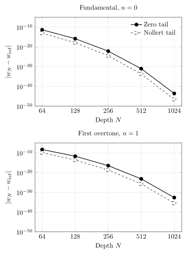
At fixed 50-digit arithmetic, increasing continued-fraction depth reduces the absolute frequency difference from the deeper reference for both Schwarzschild axial gravitational modes, with $\ell=2$ and $w=GM\omega$. The two-term Regge–Wheeler Nollert tail improves these cases. Points are computed differences, not certified bounds; joining segments guide the eye. Both axes are logarithmic and both panels use the same scales.

At fixed $N=1024$, the largest change among the two modes and two tails is $3.81\times10^{-31}$ when increasing precision from 30 to 50 digits, and $6.15\times10^{-51}$ from 50 to 80. This small arithmetic drift does not remove the larger depth error in the first overtone.

All 60 finite equations were solved, but only 18 rows passed the declared $10^{-25}$ frequency-difference, independently deep fraction, cross-inversion and matching-row tests; the other 42 remain in the results with their insufficient-accuracy labels. At $n=1$, $N=64$, zero tail and 80 digits, the solver residual is about $1.33\times10^{-79}$ while the frequency difference is $4.76\times10^{-9}$. The deep normalized fraction residual is $1.68\times10^{-8}$ and the matching-row residual is $1.86\times10^{-6}$. This is a precise solution of an insufficiently deep fraction.

The stored initial, ordinary and far-boundary rows have maximum non-matching residual below $3.2\times10^{-90}$; the independently tested matching row need not. The driver retains the coefficient values, not just a claimed residual. Its low-mode windows reject substituting the fundamental for the first overtone. Cross-inversion checks verify the equivalent fraction, not overtone identity; these tests do not label arbitrary roots outside the two stated cases.

The coupled Kerr example

Fresh solves at nine spins from $a_*=0$ to $0.4$ track the $s=-2$, $(\ell,m,n)=(2,1,0)$ mode. The final result, rounded to twelve decimal places, is

$$\begin{aligned} w&=0.407979108715-0.087257144736i,\\ A&=3.767574385986+0.053240584492i. \end{aligned}$$

The independent radial fraction evaluated at the unrounded double-precision inputs approaches $|F_0|\simeq2.0\times10^{-14}$. Its change from depth 512 to 1024 is about $9.3\times10^{-31}$: this bounds that depth change, not the error of the double-precision frequency.

A two-component example shows why an internal matrix residual is not enough. For the dimensionless toy matrix

$$H_{\rm toy}=\begin{pmatrix}4&b\\ b&10\end{pmatrix},\qquad b\gt0,$$

retaining only the first component gives $A=4$ and zero internal residual. But the same coefficient, zero-padded to two components, gives

$$(H_{\rm toy}-4I)\begin{pmatrix}1\\0\end{pmatrix} =\begin{pmatrix}0\\ b\end{pmatrix}.$$

The discarded equation has residual $b$, despite an exact retained solve. This illustrates truncation, not a Kerr frequency-error estimate.

The actual angular re-solves give the following results. The last column is the absolute Euclidean norm of the residual in the omitted rows, with the coefficient vector normalized to one; it is not the full normalized $\eta_{\rm ext}$.

Retained maximum harmonic $L$	Omitted-row residual
4	$5.43\times10^{-4}$
6	$2.57\times10^{-7}$
8	$5.30\times10^{-11}$
10	$6.10\times10^{-15}$
12	$4.47\times10^{-19}$

At $L=4$, the residual inside the retained block is already about $9\times10^{-16}$. It does not reveal the missing angular components. The full enlarged-space residual eventually reaches a floating-point floor; the continued decrease of omitted rows alone does not remove that floor.

Leaver’s Table 3 at $a_{\rm L}=0.2$ gives $\omega_{\rm L}=0.815958-0.174514i$ and $A=3.76757+0.05324i$. Since his length unit is $2GM$, $a_*=2a_{\rm L}$ and $w=\omega_{\rm L}/2$. The computed values reproduce every printed digit after this conversion; the six-decimal table cannot verify the additional digits reported by the driver. Leaver 1985, Table 3, p. 296.

The physical frequency and decay time follow from the chosen mass:

$$\omega=\frac{w}{GM},\qquad f_{\rm osc}=\frac{\operatorname{Re}w}{2\pi GM}, \qquad \tau=-\frac{GM}{\operatorname{Im}w}.$$

Rejection tests and limitations

Wrong overtone or poor seed. Root solvers follow attraction basins, not labels. Continue from independently identified low modes, inspect neighboring inversions and seed perturbations, and reject a converged root whose identity differs from the requested one. The benchmark covers only its named modes.

Wrong angular branch. Check the continued eigenvector, the eigenvalue gap and angular resolution, then re-evaluate the radial condition with that same $A$. A radial zero with an unrelated spheroidal eigenvalue is not the intended separated mode.

Finite-fraction roots. A tiny residual at one depth can certify the wrong finite problem. Require stability across at least three depths and test a deeper fraction. An asymptotic tail does not exempt a calculation from this check.

Singular and near-extremal cases. Vanishing recurrence coefficients, small elimination pivots, algebraically special frequencies and Stokes limits can invalidate a ratio or cancel factors used in an inversion. Closely separated Kerr horizons also make the usual expansion slow. The finite scripts do not certify these regimes; use regularized recurrences or a method adapted to the limiting geometry, not an unchecked increase in the number of printed digits.

Accuracy versus completeness. These checks support specific isolated roots, not an exhaustive search, a theorem about every overtone, or completeness of a quasinormal expansion. Interpretation of the resulting poles belongs to Completeness, Excitation, and Ringdown Content.

Exercises

Check the ratio index

For the toy sequence $a_j=1/(j+1)$, evaluate $R_1$. Compare the correctly shifted backward formula with the formula that incorrectly uses $(\alpha_1,\beta_1,\gamma_1)$ beside $R_2$. Does minimality make the endpoint sum finite?

Solution

Here $R_1=2/3$ and $R_2=3/4$. Row two gives

$$-\frac{\gamma_2}{\beta_2+\alpha_2R_2} =-\frac{2}{-6+4(3/4)}=\frac23.$$

Using row one instead gives $-1/[-4+3(3/4)]=4/7$, which is wrong. The sequence is minimal relative to the constant solution, but its sum at $z=1$ is the divergent harmonic series. A relative sequence comparison and an endpoint convergence test answer different questions.

Diagnose an angular calculation

A unit-norm vector has retained-block residual $9\times10^{-16}$ but omitted-row residual $5.4\times10^{-4}$. Can its angular accuracy be claimed to be near machine precision? What changes if the root is printed with sixty digits after evaluating a continued fraction at sixty-digit arithmetic?

Solution

No. The vector solves the finite matrix problem closely but fails the enlarged angular equation at the displayed omitted-row scale. Increase angular resolution and re-solve the coupled problem; monitor both retained and omitted residuals and the change in $(w,A)$. A small residual still needs a conditioning estimate before becoming an eigenvalue-error bound.

Evaluating a residual at sixty-digit arithmetic does not recover digits absent from a double-precision input. It helps separate evaluation error from the residual of that input. To claim more frequency digits, solve again at increased precision and repeat the independent depth, angular-resolution and branch checks.

References

• Leaver, E. W. (1985). “An analytic representation for the quasi-normal modes of Kerr black holes.” Proceedings of the Royal Society of London A 402(1823), 285–298. DOI. Open PDF.
• Nollert, H.-P. (1993). “Quasinormal modes of Schwarzschild black holes: The determination of quasinormal frequencies with very large imaginary parts.” Physical Review D 47, 5253–5258. DOI. Open PDF.
• Stein, L. C. (2019). “qnm: A Python package for calculating Kerr quasinormal modes, separation constants, and spherical-spheroidal mixing coefficients.” Journal of Open Source Software 4(42), 1683. DOI.