The Regge–Wheeler Equation

Odd-parity, or axial, Schwarzschild perturbations look at first like a coupled set of Einstein equations for several metric amplitudes. For every spherical harmonic with $\ell\geq2$, gauge invariance and the constraint equations reduce that set to one scalar field. This page derives its Regge–Wheeler wave equation, fixes the tortoise and Fourier conventions, and derives the physical energy normalization independently from the quadratic Einstein action and the radiation metric. The energy balance distinguishes finite portions of the future horizon and null infinity from the whole future. The propagation and reconstruction statements are linear; gravitational radiation energy is retained to leading quadratic order in a weak perturbation.

Required background. PDEs and Green Functions for Gravitation supplies the hyperbolic operator, characteristic, and conserved-current tools used below.

Helpful background. Black-Hole Geometry and Mechanics fixes the Schwarzschild exterior and its null boundaries; Formulations of General Relativity separates constraints from evolution; Presymplectic Potentials and Currents prepares the flux interpretation; Black-Hole Perturbation Theory supplies the surrounding perturbative framework.

Axial harmonics and the invariant field

Write the Schwarzschild metric as

$$ds^2=-f\,dt^2+f^{-1}dr^2+r^2d\Omega^2, \qquad f=1-\frac{2GM}{r},$$

and let lower-case Latin indices refer to the two-dimensional orbit space $(t,r)$. On the unit sphere, let $D_A$ be the covariant derivative, $\Omega_{AB}$ the metric and $\epsilon_{\theta\phi}=\sin\theta$. From scalar harmonics of unit integral norm define

$$D^AD_AY^{\ell m}=-\ell(\ell+1)Y^{\ell m},\qquad X_A^{\ell m}=-\epsilon_A{}^BD_BY^{\ell m},\qquad X_{AB}^{\ell m}=D_{(A}X_{B)}^{\ell m}.$$

Parentheses have weight one-half. These derivative-normalized vector and trace-free tensor harmonics do not themselves have unit norm. An odd-parity metric perturbation of one $(\ell,m)$ mode has

$$p_{aB}=h_a X_B^{\ell m}, \qquad p_{AB}=h_2 X_{AB}^{\ell m}.$$

The axial vector and tensor harmonics change by $(-1)^{\ell+1}$ under parity. On this page $\xi=-\xi_{\text{Ch. 1}}$ is the inverse-identification generator. The following minus-sign rule is therefore equivalent to Chapter 1’s active-plus convention after that change of generator.

An odd gauge generator $\xi X_A^{\ell m}$ acts as

$$h_a\mapsto h_a-\nabla_a\xi+\frac{2r_a}{r}\xi, \qquad h_2\mapsto h_2-2\xi,$$

where $r_a=\nabla_a r$. The cancellation is immediate in

$$\widetilde h_a =h_a-\frac12r^2\nabla_a\!\left(\frac{h_2}{r^2}\right).$$

Thus choosing Regge–Wheeler gauge, $h_2=0$, is optional: it makes $\widetilde h_a=h_a$ but does not define the physics. For $\ell\geq2$, set $\mu_\ell\equiv(\ell-1)(\ell+2)=2\lambda$, where $\lambda$ is the angular factor used in the chapter overview and on the Zerilli page. Choose the orbit-space volume form induced by the site’s four-dimensional orientation and the positive orientation of the unit sphere. In Schwarzschild coordinates,

$$\epsilon_{tr}=+1,\qquad \epsilon^{tr}=-1,\qquad t^a=-\epsilon^{ab}r_b=(\partial_t)^a.$$

This fixes the overall sign in the Cunningham–Price–Moncrief normalization

$$\Psi^{\ell m}_{\mathrm{odd}} =\frac{2r}{\mu_\ell}\epsilon^{ab} \left(\nabla_a\widetilde h_b-\frac{2r_a}{r}\widetilde h_b\right).$$

This is a scalar under changes of the orbit-space coordinates and invariant under the odd gauge transformation. The construction, including the sourced field equations, is given covariantly in Martel and Poisson 2005, § V, pp. 6–7, PDF. The original calculation instead fixed a convenient gauge and identified the single axial wave amplitude Regge and Wheeler 1957, pp. 1063–1069.

From the Einstein equations to the potential

It is worth doing the reduction rather than merely quoting its outcome. Write $L=\ell(\ell+1)$ and suppress the $(\ell,m)$ label. With the harmonic normalization used above, let $\Box_2=g^{bc}\nabla_b\nabla_c$ denote the orbit-space rough wave operator, acting on the scalar or one-form that follows it. The two odd-parity projections of the linearized Einstein equation are

$$\begin{aligned} \mathcal E_a[\widetilde h]={}& -\Box_2\widetilde h_a+\nabla_a\nabla_b\widetilde h^b +\frac{2}{r}\left( r_b\nabla_a\widetilde h^b-r_a\nabla_b\widetilde h^b \right)\\ &-\frac{2}{r^2}r_a r_b\widetilde h^b +\frac{L}{r^2}\widetilde h_a, \qquad \mathcal E[\widetilde h]=\nabla_a\widetilde h^a. \end{aligned}$$

With first-order stress–energy $T_{(1)}^{\mu\nu}$, these left-hand sides equal the source projections $\mathcal P_a=g_{ab}\mathcal P^b$ and $\mathcal P$, where

$$\begin{aligned} \mathcal P_{\ell m}^{a} &=\frac{16\pi G r^2}{L} \int T_{(1)}^{aB}\overline X_B^{\ell m}\,d\Omega,\\ \mathcal P_{\ell m} &=\frac{16\pi G r^4}{\mu_\ell L} \int T_{(1)}^{AB}\overline X_{AB}^{\ell m}\,d\Omega. \end{aligned}$$

Both source projections vanish on a vacuum open set. The vector equation comes from the $aB$ components; the scalar equation comes from the odd, trace-free part of the $AB$ components. They are linked by the projected linearized Bianchi identity

$$\nabla_a\mathcal E^a +\frac{2}{r}r_a\mathcal E^a -\frac{\mu_\ell}{r^2}\mathcal E=0.$$

Thus the displayed equations contain a constraint as well as evolution; two components of $\mathcal E_a=0$ are not two independent wave equations.

Now set

$$Q=\epsilon^{ab}\left( \nabla_a\widetilde h_b-\frac{2r_a}{r}\widetilde h_b \right), \qquad \Psi_{\mathrm{odd}}=\frac{2r}{\mu_\ell}Q.$$

The curl is the useful projection because the Hessian of a scalar is symmetric: $\epsilon^{ca}\nabla_c\nabla_a(\nabla_b\widetilde h^b)=0$. Expand the curl of the remaining terms using

$$\nabla_a\nabla_b r=\frac{GM}{r^2}g_{ab}, \qquad R_{abcd}=\frac{2GM}{r^3} (g_{ac}g_{bd}-g_{ad}g_{bc}), \qquad \nabla_a\epsilon_{bc}=0.$$

After the product rule, the second-derivative curl and the radial first-derivative terms assemble into $\Box_2(rQ)$; commuting derivatives of $\widetilde h_a$ supplies the orbit-space curvature term. Term by term, the result is the exact reduction identity

$$\begin{aligned} -\frac{2r}{\mu_\ell}\epsilon^{ca}\nabla_c\mathcal E_a &=\left( \Box_2-\frac{L}{r^2}+\frac{6GM}{r^3} \right)\left(\frac{2r}{\mu_\ell}Q\right)\\ &=\left( \Box_2-\frac{\ell(\ell+1)}{r^2}+\frac{6GM}{r^3} \right)\Psi_{\mathrm{odd}}. \end{aligned}$$

No perturbed field equation has been used in this identity; only the exact Schwarzschild background relations have. Setting $\mathcal E_a=0$ therefore gives

$$\left(\Box_2-\frac{\ell(\ell+1)}{r^2} +\frac{6GM}{r^3}\right)\Psi_{\mathrm{odd}}=0.$$

More generally, substituting $\mathcal E_a=\mathcal P_a$ into the same identity gives

$$\left(\Box_2-\frac{\ell(\ell+1)}{r^2} +\frac{6GM}{r^3}\right)\Psi_{\mathrm{odd}} =-\frac{2r}{\mu_\ell}\epsilon^{ab}\nabla_a\mathcal P_b.$$

For a distributional source, the derivative on the right and the master field must be interpreted distributionally and matched to the correct jumps; that analysis belongs on Sourced Master Equations and Junction Conditions.

Conversely, a smooth vacuum master solution reconstructs the invariant metric locally by

$$\widetilde h_a=\frac12\epsilon_{ab}\nabla^b(r\Psi_{\mathrm{odd}}).$$

Its scalar constraint vanishes identically: the divergence contracts an antisymmetric volume form with the Hessian of $r\Psi_{\mathrm{odd}}$. Substitution into the master definition returns the original field precisely when its wave equation holds; the vector equations then vanish too. Thus there is no extra local scalar constraint to impose on this full master solution. Choosing a metric gauge and selecting globally admissible boundary data remain separate tasks. Odd-Parity Metric Perturbations gives both directions explicitly. The projected system and master definition are Martel and Poisson 2005, § V.B–C, eqs. (5.8)–(5.16), pp. 6–7, PDF.

Cunningham–Price–Moncrief versus Regge–Wheeler

The field called the “Regge–Wheeler function” in older metric-component calculations is related to, but is not identical with, the radiation-adapted field used here. In the same harmonic convention define

$$\Psi_{\mathrm{RW}}=\frac1r r^a\widetilde h_a =\frac{f}{r}\widetilde h_r.$$

In Regge–Wheeler gauge this is $fh_r/r$, often written $fh_1/r$. The projected Einstein equations give

$$\Psi_{\mathrm{RW}} =\frac12 t^a\nabla_a\Psi_{\mathrm{odd}} +\frac{r}{\mu_\ell}r_a\mathcal P^a.$$

Thus in a vacuum Schwarzschild region, where $t^a\nabla_a=\partial_t$,

$$\Psi_{\mathrm{RW}}=\frac12\partial_t\Psi_{\mathrm{odd}}, \qquad \psi_{\mathrm{RW}}=-\frac{i\omega}{2}\psi_{\mathrm{odd}}$$

for $e^{-i\omega t}$ modes. The two fields satisfy the same homogeneous Regge–Wheeler operator, but their source and radiative dictionaries differ. The frequency-domain relation cannot be inverted by dividing by $\omega$ in the static sector: time differentiation loses stationary information. The full CPM inverse above retains it without division by frequency. See Martel and Poisson 2005, § V.D, Eqs. (5.17)–(5.18), p. 7, PDF.

The tortoise coordinate and axial barrier

In Schwarzschild coordinates the scalar wave operator is

$$\Box_2\Psi=-f^{-1}\partial_t^2\Psi +\partial_r\!\left(f\partial_r\Psi\right).$$

Introduce the tortoise coordinate by $dr_*/dr=f^{-1}$. In the exterior,

$$r_*=r+2GM\log\!\left(\frac{r}{2GM}-1\right)+C,$$

so $r_*\to-\infty$ at the future-horizon end and $r_*\to+\infty$ at spatial infinity. Because $f\partial_r=\partial_{r_*}$, multiplying the covariant equation by $f$ gives

$$\left[-\partial_t^2+\partial_{r_*}^2-V_{\mathrm{RW}}(r)\right] \Psi_{\mathrm{odd}}=0,$$

with

$$V_{\mathrm{RW}}(r) =f\left[\frac{\ell(\ell+1)}{r^2}-\frac{6GM}{r^3}\right].$$

This derivation also explains both terms: angular gradients supply the centrifugal barrier, while background curvature shifts it by $-6GMf/r^3$. The potential vanishes at either end of the tortoise line. For $\ell\geq2$ and $r>2GM$ it is nonnegative, since $\ell(\ell+1)r-6GM>0$ there.

A useful independent check is dimensional. In units with $c=1$, both $\partial_{r_*}^2$ and $V_{\mathrm{RW}}$ have dimensions of inverse length squared; every term in the brackets has that dimension. A second check is structural: the $m$ label never appears in the radial operator because the background is spherically symmetric. Degeneracy in $m$ is therefore a symmetry statement, not an approximation made during separation.

The physically normalized master action

A wave equation does not determine the overall coefficient of its action. That coefficient matters when the master energy is interpreted as gravitational energy. We now fix it from the Einstein–Hilbert action, before using any radiation formula. Work with one real, unit-normalized scalar sphere harmonic and its real metric amplitudes; a real basis is equivalent to the complete complex-harmonic expansion used below.

Let $g(\eta)=g+\eta p+O(\eta^2)$ on the vacuum background and define $S^{(2)}$ as the coefficient of $\eta^2$. With compactly supported variations, or with the corresponding boundary terms kept separately, the first variation of $S_{\mathrm{EH}}=(16\pi G)^{-1}\int R\sqrt{-g}\,d^4x$ gives

$$S^{(2)}_{\mathrm{EH}} =-\frac{1}{32\pi G}\int p_{\mu\nu}\,\delta G^{\mu\nu}[p]\sqrt{-g}\,d^4x.$$

The factor $1/2$ is the Taylor-series factor. The minus sign arises because the varied variable is the covariant metric. In Regge–Wheeler gauge, $p_{aB}=h_aX_B$ is the only nonzero amplitude. The Einstein projection above means $\delta G_{aB}=\mathcal E_aX_B/2$, while $\int X_AX^A\,d\Omega=L$. The two equal mixed-index contractions cancel the projection’s $1/2$; the area factor $r^2$ cancels the inverse angular metric. Since $\sqrt{-g_2}=1$ in $(t,r)$, the result is

$$S^{(2)}_{\mathrm{EH}} =-\frac{L}{32\pi G}\int dt\,dr\;h^a\mathcal E_a[h] \quad\text{up to the chosen boundary representative}.$$

From the metric one-form to a scalar

Set $A_a=\widetilde h_a/r^2$, $F_{ab}=\nabla_aA_b-\nabla_bA_a$, and $N_\ell=L/(16\pi G)$. Reorganizing the displayed Einstein operator gives

$$\mathcal E_a =-\frac{1}{r^2}\nabla_b(r^4F^b{}_a)+\mu_\ell A_a.$$

One integration by parts therefore gives the two-dimensional massive-vector action, also called a Proca action,

$$S_A=N_\ell\int dt\,dr \left[-\frac{r^4}{4}F_{ab}F^{ab} -\frac{\mu_\ell r^2}{2}A_aA^a\right].$$

More precisely, the preceding Hessian density equals this density plus $\nabla_b(N_\ell r^4A_aF^{ba}/2)$. This identifies the boundary term, not just the bulk equation. The dimensionally reduced massive-vector structure is independently obtained in Ripley and Yagi 2018, § IV.B, eqs. (40)–(50), pp. 7–8, PDF; the absolute normalization here follows from the explicit Einstein–Hilbert coefficient above.

In two dimensions an antisymmetric field strength has only one independent component. Define

$$w=\epsilon^{ab}\nabla_aA_b=\frac{Q}{r^2},\qquad F_{ab}=-\epsilon_{ab}w.$$

Replace the term $r^4w^2/2$ by a first-order expression involving an independent scalar $B$:

$$\mathcal L_1=N_\ell\left[ B\epsilon^{ab}\nabla_aA_b-\frac{B^2}{2r^4} -\frac{\mu_\ell r^2}{2}A_aA^a\right].$$

Varying $B$ gives $B=r^4w$ and recovers $S_A$. Alternatively, integrate the first term by parts. Its boundary term is $\nabla_a(N_\ell B\epsilon^{ab}A_b)$; the remaining equation for $A_a$ is algebraic:

$$A_a=\frac{\epsilon_{ab}\nabla^bB}{\mu_\ell r^2},\qquad \mathcal L_B=-\frac{N_\ell}{2} \left[\frac{\nabla_aB\nabla^aB}{\mu_\ell r^2} +\frac{B^2}{r^4}\right].$$

Eliminating this algebraic variable is legitimate in the action; substituting a solution of the propagating wave equation into an action would not be the same operation. Now $B=r^2Q=\mu_\ell r\Psi_{\mathrm{odd}}/2$. After this change of variable, define

$$C_\ell=\frac{N_\ell\mu_\ell}{4} =\frac{L\mu_\ell}{64\pi G} =\frac{1}{64\pi G}\frac{(\ell+2)!}{(\ell-2)!}.$$

Expanding $\nabla(r\Psi)$ and integrating its radial cross term yields

$$\mathcal L_B =-\frac{C_\ell}{2}\left[ \nabla_a\Psi\nabla^a\Psi +\left(\frac{L}{r^2}-\frac{6GM}{r^3}\right)\Psi^2\right] -\partial_r\!\left(\frac{C_\ell f\Psi^2}{2r}\right).$$

Here and below $\Psi=\Psi_{\mathrm{odd}}$. The total derivatives specify which boundary representative is being used; metric and scalar Dirichlet conditions on arbitrary finite boundaries are not automatically equivalent. Choosing the displayed scalar bulk representative and using $dr=f\,dr_*$ finally gives

$$S_{\mathrm{CPM}}^{(2)} =\frac{C_\ell}{2}\int dt\,dr_* \left[(\partial_t\Psi)^2-(\partial_{r_*}\Psi)^2 -V_{\mathrm{RW}}\Psi^2\right].$$

Thus the coefficient is fixed by gravity, not fitted to a later flux formula. The following energies refer to this canonical scalar representative; an arbitrary finite-boundary gravitational energy can differ by boundary terms.

Boundary orientation and finite-cut energy

Write $x=r_*$. For real nonzero frequency with time dependence $e^{-i\omega t}$, the leading future-horizon ingoing wave is $e^{-i\omega(t+x)}$, and the leading future-null-infinity outgoing wave is $e^{-i\omega(t-x)}$. These phases fix wave orientation. At zero frequency they do not form a wave basis; for complex frequency a leading exponential alone does not define the continued retarded boundary solution. That selection is developed on Chandrasekhar Transformations and Isospectrality.

For a real vacuum solution, temporarily divide the canonical energy by $C_\ell$ and set $V=V_{\mathrm{RW}}$. Define the energy density and the signed product

$$e=\frac12(\Psi_t^2+\Psi_x^2+V\Psi^2),\qquad q=\Psi_t\Psi_x,\qquad \partial_te=\partial_xq.$$

The last equality follows by multiplying the wave equation by $\Psi_t$; stationarity of $V$ is essential. On a fixed interval $[a,b]$,

$$E_{[a,b]}(t)=\int_a^b e\,dx,\qquad \frac{dE_{[a,b]}}{dt}=[q]_a^b.$$

For an outgoing field $F(u)$, $u=t-x$, the right product is $q=-F'^2$. For an ingoing field $H(v)$, $v=t+x$, the left product is $q=+H'^2$, but the bracket subtracts it. Both remove energy from the exterior. On the complete tortoise line at each finite $t$, compactly supported initial data instead have vanishing endpoint terms by finite propagation. That complete-line energy is conserved: taking spatial endpoints to infinity at fixed time is not taking a future null-boundary limit.

Spacelike slices reaching finite null cuts

To state a finite future-boundary balance precisely, choose any fixed $b_0>0$ and the spacelike slices

$$\Sigma_\tau:\quad t=\tau+h(x),\qquad h(x)=\sqrt{x^2+b_0^2},\qquad h'(x)=\frac{x}{\sqrt{x^2+b_0^2}}.$$

Because $|h'|\lt1$, these are spacelike. At the right end $h-x\to0$, so the slice meets $\mathscr I^+$ at $u=\tau$; at the left end $h+x\to0$, so it meets $\mathcal H^+$ at $v=\tau$. Two slices therefore bound only the segments between their two cuts, not either entire future boundary.

The conserved one-form $e\,dx+q\,dt$ pulls back to a positive slice energy with the coordinate measure $dx$:

$$E_\Sigma(\tau)=\int_{\mathbb R}\rho(\tau,x)\,dx,\qquad \rho=(e+h'q)\big|_{t=\tau+h(x)}.$$

The cross term accounts for the tilted slice; replacing this density by $e$ would integrate a different quantity. For $\varphi(\tau,x)=\Psi(\tau+h(x),x)$ it is equivalently

$$\rho=\frac12\left[ \frac{b_0^2}{x^2+b_0^2}\varphi_\tau^2 +\varphi_x^2+V\varphi^2\right]\geq0.$$

Positivity uses $V\geq0$; the coefficient of $\varphi_\tau^2$ tends to zero at the ends, so this is not uniform control of its unweighted norm. First truncate at $x=\pm R$, calling the integral $E_{\tau,R}$. Conservation gives the exact identity

$$\begin{aligned} E_{\tau_2,R} &+\int_{\tau_1}^{\tau_2} \left[-q(\tau+h(R),R)+q(\tau+h(R),-R)\right]d\tau\\ &=E_{\tau_1,R}. \end{aligned}$$

For a sufficient limiting hypothesis, suppose the slice energies are finite and the derivative pairs have strong $L^2([\tau_1,\tau_2])$ limits

$$\begin{aligned} (\Psi_t,\Psi_x)(\tau+h(R),R)&\longrightarrow(F'(\tau),-F'(\tau)),\\ (\Psi_t,\Psi_x)(\tau+h(R),-R)&\longrightarrow(H'(\tau),H'(\tau)). \end{aligned}$$

Then the products converge in $L^1$, and positivity permits the limit of the truncated energies. The resulting finite-cut balance is

$$E_\Sigma(\tau_2) +\int_{\tau_1}^{\tau_2}F'(u)^2\,du +\int_{\tau_1}^{\tau_2}H'(v)^2\,dv =E_\Sigma(\tau_1).$$

Here $F'$ and $H'$ are the radiation derivative traces; integrating them defines profiles $F,H$ up to additive constants. If the field traces also exist, choose these profiles to equal the limiting fields. Derivative convergence alone does not establish that additional fact. The stated derivative limits, not merely $V\to0$, justify the flux calculation. Multiplying every energy and flux by $C_\ell$ restores the physical canonical normalization.

In the diagram, follow each slice to its two labeled cuts. The gray shading marks the spacetime region between the slices, not an energy density. Only the heavy boundary segments enter the finite-cut balance; the thin continuations belong to later cuts. The short flux arrows point out of the exterior and end at its boundaries, rather than indicating motion along them.

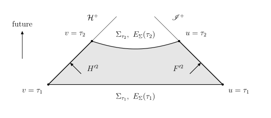
Two spacelike slices enclose finite portions of the future horizon and null infinity. For $t=\tau+\sqrt{x^2+b_0^2}$, their endpoint cuts satisfy $v=\tau$ on $\mathcal H^+$ and $u=\tau$ on $\mathscr I^+$; the illustrated pair has $\tau_1=0$ and $\tau_2=b_0$. Under the derivative-trace assumptions stated above, energy crossing the highlighted segments accounts for the difference between the slice energies. Schematic compactification of the exterior only; the diagram does not assert complete decay.

If these hypotheses hold for all later finite cuts, a second limit gives

$$E_\Sigma(\tau_1) =E_{\mathrm{rem}} +\int_{\tau_1}^{\infty}F'(u)^2\,du +\int_{\tau_1}^{\infty}H'(v)^2\,dv,\qquad E_{\mathrm{rem}}=\lim_{\tau\to\infty}E_\Sigma(\tau)\geq0.$$

Eliminating the residual energy requires a separate decay or completeness result; this local balance does not prove it. The free-pulse exercise below checks the finite limits explicitly.

Matching the radiation metric

There is an independent way to determine the coefficient. In a vacuum neighborhood of future null infinity, an outgoing radiation gauge gives

$$p_{AB}^{\mathrm{rad,odd}} =r\sum_{\ell m}\Psi_{\mathrm{odd}}^{\ell m}(u,\infty) X_{AB}^{\ell m}+O(1).$$

With indices raised by the unit-sphere metric,

$$\int \overline X^{AB}_{\ell m}X_{AB}^{\ell' m'}\,d\Omega =\frac{L\mu_\ell}{2}\delta_{\ell\ell'}\delta_{mm'}.$$

The vector and tensor norms are Martel and Poisson 2005, § III, eqs. (3.4) and (3.9), p. 3, PDF. The angular metric coefficients $p_{AB}$ are not dimensionless strains: two inverse physical angular metrics are required in the contraction. The transverse-traceless radiation formula is

$$\left\langle\frac{dE_\infty^{\mathrm{odd}}}{du}\right\rangle =\lim_{r\to\infty}\frac{r^2}{32\pi G} \int_{S^2}\left\langle \partial_up_{AB}^{\mathrm{rad,odd}} \partial_up_{CD}^{\mathrm{rad,odd}} \right\rangle \frac{\Omega^{AC}\Omega^{BD}}{r^4}\,d\Omega.$$

The metric amplitudes contribute $r^2$, the two inverse metrics contribute $r^{-4}$, and the area contributes $r^2$. The remaining harmonic norm gives

$$\left\langle\frac{dE_\infty^{\mathrm{odd}}}{du}\right\rangle =\sum_{\ell m}C_\ell \left\langle\left|\partial_u\Psi_{\mathrm{odd}}^{\ell m}\right|^2 \right\rangle\geq0.$$

This is exactly the coefficient derived from the quadratic Einstein action. The brackets denote a radiation time average; before such averaging, the same squared-derivative expression is the positive canonical boundary power. The metric relation and averaged radiation flux are Martel and Poisson 2005, § VI, eqs. (6.12) and (6.16), pp. 8–9, PDF.

For a real perturbation expanded in complex harmonics, $\Psi^{\ell,-m}=(-1)^m\overline{\Psi^{\ell m}}$, and the displayed sum runs over all $m=-\ell,\ldots,\ell$. It already includes both members of each reality pair: do not insert another factor of one-half. By contrast, if a single real mode is written as $\Psi=\operatorname{Re}(a e^{-i\omega u})$ with real $\omega\ne0$, its period average has $\langle\Psi_u^2\rangle=\omega^2|a|^2/2$. This is a time-average factor, not an angular-pairing factor.

Horizon absorption and its interpretation

The horizon comparison uses a vacuum neighborhood, a regular horizon-locking radiation gauge, and $r_+=2GM$. Here the odd angular metric has the opposite sign from its infinity expression:

$$p_{AB}^{\mathcal H,\mathrm{odd}} =-r_+\sum_{\ell m}\Psi_{\mathrm{odd}}^{\ell m}(v,r_+)X_{AB}^{\ell m}.$$

Its first-order shear is $\sigma_{AB}=\partial_vp_{AB}^{\mathcal H}/2$. The minus sign matters for metric reconstruction but disappears in the shear squared. Raising indices with $r_+^{-2}\Omega^{AB}$ twice and using $dA=r_+^2d\Omega$ yields

$$\frac{1}{8\pi G}\int_{\mathcal H_v}\sigma_{AB}\sigma^{AB}\,dA =\sum_{\ell m}C_\ell \left|\partial_v\Psi_{\mathrm{odd}}^{\ell m}\right|^2.$$

This is a shear/area calculation, not the large-radius TT approximation applied at the horizon. At leading quadratic order the vacuum Raychaudhuri equation is

$$\partial_v\vartheta=\kappa\vartheta-\sigma_{AB}\sigma^{AB},\qquad \kappa=\frac{1}{4GM}.$$

For weak perturbations with settled stationary endpoints, the endpoint expansions vanish. Integrating this equation and using the perturbative first law gives

$$\Delta E_{\mathcal H}=\frac{\kappa\,\Delta A}{8\pi G} =\frac{1}{8\pi G}\int dv\int_{\mathcal H_v} \sigma_{AB}\sigma^{AB}\,dA.$$

Equivalently, an average long compared with $\kappa^{-1}$ can neglect the endpoint transient and identifies the corresponding averaged absorption rate. On arbitrary finite cuts there is an expansion endpoint term: the exact canonical flux in the preceding section must not be called a definition-independent instantaneous black-hole mass derivative. The total change must remain perturbatively small compared with $M$; no low-frequency restriction on individual Schwarzschild modes is introduced here. The odd horizon sign and flux are Martel and Poisson 2005, § VII, eqs. (7.3)–(7.5), pp. 9–10, PDF. The gauge, shear law and endpoint/averaging assumptions are developed in Poisson 2004, § IV, pp. 10–12, and § VI.A, pp. 17–18, PDF.

Domain, checks, and limitations

The radiative statement starts at $\ell=2$. The odd monopole does not exist, and the odd dipole contains the linearized angular-momentum perturbation plus gauge, rather than a Regge–Wheeler gravitational wave. Near either asymptotic end $V_{\mathrm{RW}}\to0$, providing an immediate check of the null-wave orientations. The flat limit $GM\to0$ leaves the spherical centrifugal barrier, another dimensional and physical check.

This page derives the vacuum master equation, its physical canonical normalization and its finite-cut energy balance under explicit radiation-limit hypotheses. Localized matter changes the right-hand side and requires junction conditions. Spectral solution methods remain in the later response chapters, while generic numerical implementation belongs to Computational Relativity.

Exercises

Curl the projected Einstein equation

In Schwarzschild coordinates set

$$C=\partial_r\widetilde h_t-\partial_t\widetilde h_r -\frac{2}{r}\widetilde h_t=Q.$$

Starting from the projected vector equation, show that

$$\begin{aligned} \mathcal E^r &=-\partial_tC+\frac{\mu_\ell f}{r^2}\widetilde h_r,\\ \mathcal E^t &=\partial_rC+\frac{2C}{r} -\frac{\mu_\ell}{r^2f}\widetilde h_t. \end{aligned}$$

Take its orbit-space curl and use $C=\mu_\ell\Psi_{\mathrm{odd}}/(2r)$ to recover the vacuum Regge–Wheeler equation.

Solution

The orientation fixed above gives

$$-\epsilon^{ab}\nabla_a\mathcal E_b =f^{-1}\partial_t\mathcal E^r +f\partial_r\mathcal E^t+f'\mathcal E^t.$$

Substitute the two projected components. Terms proportional to the metric amplitudes cancel because

$$\frac{\mu_\ell}{r^2} \left( \partial_t\widetilde h_r-\partial_r\widetilde h_t +\frac{2}{r}\widetilde h_t \right) =-\frac{\mu_\ell}{r^2}C.$$

Using $\mu_\ell=L-2$, $f=1-2GM/r$, and $f'=2GM/r^2$, the remaining terms give

$$-\epsilon^{ab}\nabla_a\mathcal E_b =\left( \Box_2+\frac{2f}{r}\partial_r -\frac{L}{r^2}+\frac{8GM}{r^3} \right)C.$$

The last product-rule step is

$$\Box_2\!\left(\frac{\Psi}{r}\right) +\frac{2f}{r}\partial_r\!\left(\frac{\Psi}{r}\right) =\frac1r\Box_2\Psi-\frac{2GM}{r^4}\Psi.$$

Since $C=\mu_\ell\Psi_{\mathrm{odd}}/(2r)$, the last term changes the curvature coefficient from $8$ to $6$:

$$-\frac{2r}{\mu_\ell}\epsilon^{ab}\nabla_a\mathcal E_b =\left( \Box_2-\frac{L}{r^2}+\frac{6GM}{r^3} \right)\Psi_{\mathrm{odd}}.$$

Vacuum sets $\mathcal E_b=0$, which is the desired equation. The component equations used in this check are tabulated in Martel and Poisson 2005, Appendix C, p. 16, PDF.

Follow two pulses through finite cuts

For this exercise only, set $V=0$ on the complete $x$ line and take smooth compact profiles $F,H$ with $\Psi(t,x)=F(t-x)+H(t+x)$. This is a free-wave check of the energy geometry, not a solution of Schwarzschild scattering with its nonzero barrier. Compute $E_\Sigma(\tau)$ on the slices above. Explain why inserting the whole-future flux after $\tau_1$ into the balance between $\tau_1$ and $\tau_2$ is wrong.

Solution

Differentiation gives $\Psi_t=F'+H'$ and $\Psi_x=-F'+H'$. Their cross terms cancel in the energy and signed product:

$$e=F'^2+H'^2,\qquad q=-F'^2+H'^2,$$

and consequently

$$\rho=(1-h')F'(\tau+h-x)^2+(1+h')H'(\tau+h+x)^2.$$

For the first term change variable to $u=\tau+h-x$: as $x$ increases, $u$ decreases from infinity to $\tau$, with $du=(h'-1)dx$. For the second use $v=\tau+h+x$, which increases from $\tau$ to infinity, with $dv=(h'+1)dx$. Thus

$$E_\Sigma(\tau)=\int_\tau^\infty F'(s)^2\,ds +\int_\tau^\infty H'(s)^2\,ds.$$

Subtract the values at two cuts to recover exactly the finite-interval fluxes. Using whole-future integrals instead would give

$$E_\Sigma(\tau_2) +\int_{\tau_1}^{\infty}(F'^2+H'^2)\,ds -E_\Sigma(\tau_1)=E_\Sigma(\tau_2),$$

which need not vanish: it counts energy that has not crossed the second cut twice. In this particular compact free-pulse example $E_{\mathrm{rem}}=0$ once $\tau$ passes both supports. That explicit fact is not a proof for a different potential. Meanwhile the complete fixed-$t$ energy is $\int_{\mathbb R}(F'^2+H'^2)ds$ at every finite time. The two statements use different slices and are consistent.

Normalize one real quadrupolar pulse

Take one real unit-normalized $\ell=2$ scalar harmonic and its axial tensor harmonic. Specify an infinity profile $\Psi(u)=a\exp[-u^2/(2T^2)]$ with real $a$ and $T>0$, both of dimension length. Find its canonical boundary power and whole-pulse energy, and recover the same coefficient by contracting the radiation metric. This is a boundary-profile example, not a prediction of the horizon’s transmitted profile.

Solution

For $\ell=2$, $L=6$, $\mu_\ell=4$ and $C_2=3/(8\pi G)$. Therefore

$$P_\infty(u)=\frac{3a^2}{8\pi G T^4}u^2e^{-u^2/T^2},\qquad E_\infty=\frac{3a^2\sqrt\pi}{16\pi G T}.$$

We used $\int_{\mathbb R}u^2e^{-u^2/T^2}du=\sqrt\pi T^3/2$. The tensor norm is $L\mu_\ell/2=12$; the metric contraction hence gives $12/(32\pi G)=3/(8\pi G)$, the same coefficient as the action. A fixed normalized convolution time average preserves the whole-line integral for this integrable power profile. No additional factor of one-half is needed: the field and its derivative are already real, not complex monochromatic amplitudes awaiting a period average. The energy has dimension length$/G$, as required for an energy in $c=1$ units.

References

• Martel, K., and Poisson, E. (2005). “Gravitational perturbations of the Schwarzschild spacetime: A practical covariant and gauge-invariant formalism.” Physical Review D 71, 104003. DOI.
• Poisson, E. (2004). “Absorption of mass and angular momentum by a black hole: Time-domain formalisms for gravitational perturbations, and the small-hole/slow-motion approximation.” Physical Review D 70, 084044. DOI. Open PDF.
• Regge, T., and Wheeler, J. A. (1957). “Stability of a Schwarzschild Singularity.” Physical Review 108, 1063–1069. DOI.
• Ripley, J. L., and Yagi, K. (2018). “Black hole perturbation under 2 + 2 decomposition in the action.” Physical Review D 97, 024009. DOI. Open PDF.