Sourced Master Equations and Junction Conditions

A localized stress tensor drives a black-hole master field through delta distributions and their derivatives. A delta changes the field’s slope; a delta derivative can change the field itself. When the source moves, time derivatives also contribute to these jumps. This page constructs normalized Schwarzschild forcing, derives the fixed and moving jump conditions, and checks them against explicit retarded Green solutions. The radiative formulas apply to $\ell\geq2$ in the exterior. They do not replace metric junction conditions for a material shell or prescribe a particle’s self-force.

Required background. PDEs and Green Functions for Gravitation supplies distributions, fundamental solutions, and retarded boundary conditions.

Helpful background. Black-Hole Geometry and Mechanics fixes horizon and infinity orientations; Formulations of General Relativity supplies the constraint identities; Presymplectic Potentials and Currents prepares sourced balance laws; Black-Hole Perturbation Theory supplies the master variables.

Stress-energy projection and master normalization

Write $m=GM$, $f=1-2m/r$, and $x=r_*$ with $dx/dr=f^{-1}$. The two-dimensional orbit metric is $g_{ab}dx^a dx^b=-fdt^2+f^{-1}dr^2$; $\nabla_a$ is its covariant derivative and $r_a=\nabla_a r$. For a suppressed harmonic label $(\ell,m_{\rm sph})$, set

$$L=\ell(\ell+1),\qquad \mu=L-2,\qquad \Lambda=\mu+\frac{6m}{r},\qquad \ell\geq2.$$

Here $m_{\rm sph}$ is the azimuthal integer, not the length $m=GM$. Use unit-normalized scalar harmonics $Y$ and their derivative-normalized partners on the unit sphere:

$$\begin{aligned} Y_A&=D_A Y,& Y_{AB}&=D_A D_B Y+\frac L2\Omega_{AB}Y,\\ X_A&=-\epsilon_A{}^B D_B Y,& X_{AB}&=D_{(A}X_{B)}. \end{aligned}$$

The parentheses have weight one half. With unit-sphere index raising, the scalar norm is one, vector norms are $L$, and trace-free tensor norms are $L\mu/2$. An overbar denotes complex conjugation. For the orbit orientation use $\epsilon_{tr}=1$, so $\epsilon^{tr}=-1$. These definitions agree with Martel and Poisson 2005, § III, Eqs. (3.1)–(3.9), p. 104003-3.

Which master fields are being sourced?

Use the Zerilli–Moncrief even field and the Cunningham–Price–Moncrief (CPM) odd field, as on the preceding Zerilli and Moncrief reduction pages:

$$\begin{aligned} \Psi_+&=\frac{2r}{L}\left[ \widetilde K+\frac2\Lambda \left(r^a r^b\widetilde h_{ab}-r r^a\nabla_a\widetilde K\right) \right],\\ \Psi_-&=\frac{2r}{\mu}\epsilon^{ab} \left(\nabla_a\widetilde h_b-\frac2r r_a\widetilde h_b\right). \end{aligned}$$

For completeness, the even metric amplitudes are $p_{ab}=h_{ab}Y$, $p_{aB}=j_aY_B$, and $p_{AB}=r^2(K\Omega_{AB}Y+\mathcal GY_{AB})$. Define $\eta_a=j_a-r^2\nabla_a\mathcal G/2$; then

$$\widetilde h_{ab}=h_{ab}-\nabla_a\eta_b-\nabla_b\eta_a, \qquad \widetilde K=K+\frac L2\mathcal G-\frac2r r^a\eta_a.$$

For odd amplitudes $p_{aB}=h_aX_B$, $p_{AB}=h_2X_{AB}$, $\widetilde h_a=h_a-\nabla_a h_2/2+r_a h_2/r$. Thus the normalization is specified independently of gauge. The source formulas below correspond to precisely these fields (Martel and Poisson 2005, Eqs. (4.23), (5.13), pp. 104003-5, 104003-7).

Six projections of the physical stress tensor

Let $T^{\mu\nu}$ be the first-order physical stress tensor. Raise its indices with the physical background inverse metric, whose angular block is $r^{-2}\Omega^{AB}$, before taking these projections:

$$\begin{aligned} Q^{ab}&=8\pi G\int T^{ab}\overline Y\,d\Omega,\\ Q^a&=\frac{16\pi G r^2}{L}\int T^{aB}\overline Y_B\,d\Omega,\\ Q^{\flat}&=8\pi G r^2\int T^{AB}\Omega_{AB}\overline Y\,d\Omega,\\ Q^{\sharp}&=\frac{32\pi G r^4}{L\mu} \int T^{AB}\overline Y_{AB}\,d\Omega, \end{aligned}$$ $$P^a=\frac{16\pi G r^2}{L}\int T^{aB}\overline X_B\,d\Omega, \qquad P=\frac{16\pi G r^4}{L\mu} \int T^{AB}\overline X_{AB}\,d\Omega.$$

The even and odd tensor prefactors differ by two. Newton’s constant is already included: do not multiply the final master sources by another $8\pi G$. These are the $G$-restored projections in Martel and Poisson 2005, Eqs. (4.17)–(4.20), p. 104003-5, and Eqs. (5.10)–(5.11), p. 104003-7.

To see how point support enters, let a particle of mass $m_p$ follow $z^\mu(\tau)$ with $u^\mu=dz^\mu/d\tau$. Its stress distribution is

$$T^{\mu\nu}=m_p\int u^\mu u^\nu \frac{\delta^{(4)}(x-z(\tau))}{\sqrt{-g_4}}\,d\tau =\frac{m_p u^\mu u^\nu}{u^t r^2} \delta(r-r_p(t))\,\delta_{S^2}(\Omega,\Omega_p(t)).$$

The second expression uses exterior Schwarzschild time with $u^t\gt0$, and $\int\delta_{S^2}(\Omega,\Omega_p)q(\Omega)d\Omega=q(\Omega_p)$. For example,

$$Q^{ab}=\frac{8\pi Gm_p u^a u^b}{u^t r_p^2} \overline Y(\Omega_p)\,\delta(r-r_p).$$

The other projections follow by the same angular evaluation. Radial and time differentiation during the master reduction can turn this delta support into a delta derivative. Such a derivative does not by itself signify a material dipole layer.

Source conservation is a constraint

The first-order Bianchi identity requires $\nabla_\mu T^{\mu\nu}=0$ on the background. In these projections it is

$$\begin{aligned} \nabla_bQ^{ab}+\frac2r r_bQ^{ab} -\frac{L}{2r^2}Q^a-\frac1r r^aQ^{\flat}&=0,\\ \nabla_aQ^a+\frac2r r_aQ^a -\frac{\mu}{2r^2}Q^{\sharp}+Q^{\flat}&=0,\\ \nabla_aP^a+\frac2r r_aP^a-\frac{\mu}{r^2}P&=0. \end{aligned}$$

These are distributional identities when the matter is singular (Martel and Poisson 2005, Eqs. (4.21)–(4.22), p. 104003-5, and Eq. (5.12), p. 104003-7). A geodesic particle satisfies them. A prescribed nongeodesic particle does not generally do so by itself: stress-energy associated with the force must also be included. An arbitrary pair of functions forcing a master PDE is useful for testing that PDE, but is not automatically a consistent gravitational matter model.

From covariant sources to the tortoise equation

The covariant orbit-space equations have the form

$$(\Box_2-U_\pm)\Psi_\pm=\mathcal S_\pm, \qquad \Box_2=-f^{-1}\partial_t^2+\partial_r(f\partial_r).$$

Put $Q=g_{ab}Q^{ab}$ and $P_b=g_{ba}P^a$. Their complete forcing is

$$\mathcal S_-=-\frac{2r}{\mu}\epsilon^{ab}\nabla_aP_b,$$ $$\begin{aligned} \mathcal S_+={}&\frac4\Lambda r_aQ^a-\frac{Q^{\sharp}}r\\ &+\frac{2}{L\Lambda}\left\{ -2r^2r^a\nabla_aQ +\frac{24m}{\Lambda}r_ar_bQ^{ab} +2rfQ^{\flat}\right.\\ &\hspace{5em}\left. +\frac r\Lambda\left[ \mu(\mu-2)+12(\mu-3)\frac mr+84\frac{m^2}{r^2} \right]Q\right\}. \end{aligned}$$

These combinations result from eliminating the constrained Einstein amplitudes while retaining their stress projections; the vacuum reductions on the preceding pages set those projections to zero. The full sourced identities are given in Martel and Poisson 2005, Eq. (4.27), p. 104003-6, and Eq. (5.16), p. 104003-8. All derivatives act on the distributions as well as their smooth coefficients. Discarding a derivative of a source amplitude changes the forcing.

Multiplying the covariant equation by $f$ gives the propagation equation:

$$\mathscr L_\pm\Psi_\pm=S_\pm,\qquad \mathscr L_\pm=-\partial_t^2+\partial_x^2-V_\pm, \qquad V_\pm=fU_\pm,\qquad S_\pm=f\mathcal S_\pm.$$

A source quoted for $\Box_2-U$ cannot be inserted unchanged into $\mathscr L$. For reference, with $\lambda=\mu/2$,

$$\begin{aligned} V_-&=f\left(\frac{L}{r^2}-\frac{6m}{r^3}\right),\\ V_+&=\frac{2f}{r^3(\lambda r+3m)^2} \left[\lambda^2(\lambda+1)r^3 +3\lambda^2mr^2+9\lambda m^2r+9m^3\right]. \end{aligned}$$

There is a further distinction in the odd sector. The Regge–Wheeler field $\Psi_{\rm RW}=r^a\widetilde h_a/r$ obeys

$$\Psi_{\rm RW}=\frac12\partial_t\Psi_-+\frac r\mu P^r.$$

The correction has no additional factor of $f$ because $P^r$ is already contravariant. It vanishes in vacuum, but not generally on matter support (Martel and Poisson 2005, Eq. (5.18), p. 104003-8). See the sourced Regge–Wheeler relation for its distinct forcing. The following jump derivation assumes an ordinary piecewise smooth master field with a delta/delta-prime source. Before applying it to another master variable, check whether the variable itself contains an additional distribution concentrated on the source.

Fixed-interface jumps

Suppress parity and harmonic labels. First place an interface at a fixed $x=x_0$ and write the canonical source, whose coefficients depend only on time,

$$\mathscr L\Psi=F(t)\delta'_x(x-x_0)+G(t)\delta(x-x_0).$$

Here $G(t)$ is a source coefficient, not Newton’s constant. The delta is normalized with respect to $dx$, and its prime means $\partial_x$. Away from the source let $\Psi^\pm$ be smooth and solve the homogeneous equation; define right-minus-left traces $[q]=q^+(t,x_0)-q^-(t,x_0)$. For

$$\Psi=\Psi^-\Theta(x_0-x)+\Psi^+\Theta(x-x_0),$$

distributional differentiation gives

$$\begin{aligned} \partial_x\Psi&=(\partial_x\Psi)_{\rm pw}+[\Psi]\delta,\\ \partial_x^2\Psi&=(\partial_x^2\Psi)_{\rm pw} +[\partial_x\Psi]\delta+[\Psi]\delta'_x. \end{aligned}$$

The subscript pw means ordinary derivatives on the two open sides. Neither $\partial_t^2$ nor multiplication by smooth $V$ creates a singular term at a fixed interface. Comparing independent distributions gives

$$[\Psi]=F,\qquad [\partial_x\Psi]=G.$$

Canonical forcing at a fixed interface	Field jump	Slope jump
$G\delta$	$0$	$G$
$F\delta'_x$	$F$	$0$
$F\delta'_x+G\delta$	$F$	$G$

Integrating with a test function constant near the source isolates the delta coefficient. A test function with a prescribed first derivative also detects the delta-prime coefficient. An ordinary small-interval integral alone misses that second condition. The value assigned to $\Psi$ at the single source point changes neither distribution nor one-sided traces.

Changing the radial delta and its derivative

A coefficient multiplying $\delta(r-r_p)$ is not the coefficient multiplying $\delta(x-X)$, where $X(t)=x(r_p(t))$. Work at fixed $t$, with $r_p\gt2m$, $f_p=f(r_p)\gt0$ and $f'_p=(\partial_r f)(r_p)$. The measure transformation $dx=dr/f$ gives

$$\delta(r-r_p)=\frac{\delta(x-X)}{f_p},\qquad \delta'_r(r-r_p)=\frac{\delta'_x(x-X)}{f_p^2} +\frac{f'_p}{f_p^2}\delta(x-X).$$

The second term is essential when $f$ varies. To derive its sign, pair the left side with a smooth compactly supported test function $\varphi$ using the $dx$ measure:

$$\begin{aligned} \int\delta'_r(r-r_p)\varphi(x)\,dx &=-\left.\partial_r\left[\frac{\varphi(x(r))}{f(r)}\right]\right|_{r_p}\\ &=-\frac{\varphi_x(X)}{f_p^2} +\frac{f'_p\varphi(X)}{f_p^2}. \end{aligned}$$

There is another product rule if the radial coefficients vary in space:

$$A(t,r)\delta'_r(r-r_p) =A_p\delta'_r(r-r_p)-A_{r,p}\delta(r-r_p).$$

Consequently, transform the complete tortoise-equation source $S=A(t,r)\delta'_r+B(t,r)\delta$ to canonical form as

$$F=\frac{A_p}{f_p^2},\qquad G=\frac{B_p-A_{r,p}}{f_p}+\frac{A_pf'_p}{f_p^2}.$$

The partial derivative $A_{r,p}$ is taken before evaluating on the worldline. If starting from the covariant source $\mathcal S$, first form $S=f\mathcal S$; that factor also participates in this product rule. At a fixed interface the radial slope condition is $[\partial_r\Psi]=G/f_p$, not $G$.

Moving-interface jumps

Now let $X(t)$ be a smooth timelike interface. Set

$$v=\dot X,\qquad a=\ddot X,\qquad D=1-v^2\gt0, \qquad J=[\Psi],\qquad K=[\partial_x\Psi].$$

The traces are evaluated at $(t,X(t))$. Differentiating them follows the interface, so the chain rule is

$$\dot J=[\partial_t\Psi]+vK.$$

In the diagram, compare the direction that holds $x$ fixed with the direction tangent to the moving interface. Their difference supplies exactly the spatial term in this chain rule.

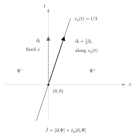
A trace follows the moving interface, whereas a partial time derivative holds $x$ fixed. Thus $\dot J=[\partial_t\Psi]+v[\partial_x\Psi]$. In the equal-scale coordinate diagram, $x_p(t)=X(t)=t/3$ and $\dot x_p=v$. It illustrates local interface kinematics, not a black-hole waveform or shell matching geometry.

For the piecewise field, $\partial_t\Theta(x-X)=-v\delta(x-X)$. Writing $H=[\partial_t\Psi]$ and reducing all coefficients to traces after differentiation gives

$$\begin{aligned} (\partial_t^2\Psi)_{\rm sing} &=v^2J\delta'_x-(2vH+aJ+v^2K)\delta,\\ (\partial_x^2\Psi)_{\rm sing}&=J\delta'_x+K\delta. \end{aligned}$$

For example, reducing a coefficient $q(t,x)\delta'_x$ uses $q\delta'_x=q_p\delta'_x-q_{x,p}\delta$; omitting this step loses part of the $v^2K$ term. Combining the derivatives and substituting $H=\dot J-vK$ yields

$$(\mathscr L\Psi)_{\rm sing} =DJ\delta'_x+\left(DK+2v\dot J+aJ\right)\delta.$$

Hence the two moving jump conditions for canonical coefficients $F(t),G(t)$ are

$$J=\frac FD,\qquad K=\frac{G-2v\dot J-aJ}{D}.$$

They determine the partial-time jump through $H=\dot J-vK$. To express everything through the source coefficients and trajectory, differentiate $J=F/D$ completely:

$$K=\frac GD-\frac{2v\dot F}{D^2} -\frac{aF(1+3v^2)}{D^3}.$$

Here $\dot F$ is the total derivative of the canonical coefficient. A stationary trajectory has $v=a=0$, recovering $J=F$, $K=G$. The factors $D^{-1}$ do not license a null-interface limit: when $D=0$ the interface is characteristic and these two noncharacteristic conditions are no longer invertible. The radial conversion also assumes $f_p\gt0$; horizon-regular source coordinates require their own transformation.

Retarded construction and direct matching

Let the retarded kernel satisfy

$$\mathscr L_xG_{\rm ret}(t,x;s,y)=\delta(t-s)\delta(x-y), \qquad G_{\rm ret}=0\quad(t\lt s).$$

For zero-past forcing with sufficient spatial support or convergence, the solution with zero past field is

$$\Psi(t,x)=\int ds\,dy\,G_{\rm ret}(t,x;s,y)S(s,y).$$

Nonzero initial field and velocity require adding the corresponding homogeneous initial-data solution. For a canonical moving source, convolution becomes, away from coincidence,

$$\Psi(t,x)=\int ds\left[ G(s)G_{\rm ret}(t,x;s,X(s)) -F(s)\left.\partial_yG_{\rm ret}(t,x;s,y)\right|_{y=X(s)} \right].$$

The derivative acts on the source coordinate and has a minus sign. Use one-sided limits instead of assigning an arbitrary derivative to a coincident kernel.

Fixed-source frequency matching

With the $e^{-i\omega t}$ inverse transform, define $\mathscr L_\omega=\partial_x^2+\omega^2-V$. For retarded inversion begin on a convergent upper-half-plane contour. Let $u_L$ be horizon-ingoing and $u_R$ infinity-outgoing, with

$$u_L\sim e^{-i\omega x}\quad(x\to-\infty),\qquad u_R\sim e^{i\omega x}\quad(x\to+\infty).$$

For $W=u_Lu_R'-u_Ru_L'\ne0$, the kernel is $g(x,y)=u_L(x_<)u_R(x_>)/W$, where $x_<=\min(x,y)$ and $x_>=\max(x,y)$. It is continuous and obeys $[\partial_xg]_y=1$, so $\mathscr L_\omega g=+\delta(x-y)$. The mode Green-function page derives this normalization and illustrates the unit jump.

Take fixed support $x_0$ and transformed coefficients $F_\omega,G_\omega$. Integrating the source gives $\psi=G_\omega g-F_\omega\partial_y g$, or explicitly

$$\psi(x)=\begin{cases} \displaystyle\frac{u_L(x)}W \left[G_\omega u_R(x_0)-F_\omega u_R'(x_0)\right],&x\lt x_0,\\[4pt] \displaystyle\frac{u_R(x)}W \left[G_\omega u_L(x_0)-F_\omega u_L'(x_0)\right],&x\gt x_0. \end{cases}$$

Subtracting the field traces cancels the $G_\omega$ terms and leaves $F_\omega W/W$. Subtracting the derivative traces cancels the $F_\omega$ terms and leaves $G_\omega W/W$. Thus this independently constructed solution obeys both jumps, the homogeneous equation on each side, and the two endpoint conditions. Zeros of $W$, analytic continuation, and noncompact forcing need the separate qualifications developed in the response chapters.

A causal moving-source example

An exact free example checks the motion terms without a numerical solver. Set $V=0$ on the whole line, $X(s)=vs$ with constant $|v|\lt1$, and let $F,G$ vanish smoothly for $s\leq0$. For the chosen sign of $\mathscr L$,

$$G_0(t,x;s,y)=-\frac12\Theta(t-s-|x-y|).$$

To the right of the trajectory, the past outgoing ray intersects the source at $s_+=(t-x)/(1-v)$; on the left the other ray intersects at $s_-=(t+x)/(1+v)$. Define $I(s)=\int_{-\infty}^sG(q)dq$. Direct convolution gives

$$\begin{aligned} \Psi^+(t,x)&=-\frac12 I(s_+)+\frac{F(s_+)}{2(1-v)},&x&\gt vt,\\ \Psi^-(t,x)&=-\frac12 I(s_-)-\frac{F(s_-)}{2(1+v)},&x&\lt vt. \end{aligned}$$

The denominators $1\mp v$ come from the delta’s retarded-root Jacobian, not from a field normalization. At the interface both retarded times approach $t$. Differentiating the branches then gives

$$J=\frac{F}{1-v^2},\qquad K=\frac{G}{1-v^2}-\frac{2v\dot F}{(1-v^2)^2},$$

exactly the general result with $a=0$. Each branch depends only on $t-x$ or $t+x$ and solves the free wave equation. Smooth switch-on ensures zero past data, so no incoming homogeneous wave has been added. This is a manufactured master-PDE check, not a Schwarzschild particle waveform or a proof that its forcing arises from conserved matter.

Energy work and the limits of singular matching

For a real field with sufficient spatial and time regularity and a smooth source, define on a finite fixed interval $[x_a,x_b]$

$$e=\frac12\left(\Psi_t^2+\Psi_x^2+V\Psi^2\right),\qquad j=-\Psi_t\Psi_x,\qquad E(t)=\int_{x_a}^{x_b}e\,dx.$$

Assume $V$ is time independent. Multiplying $-\Psi_{tt}+\Psi_{xx}-V\Psi=S$ by $\Psi_t$ and applying the ordinary product rule gives the signed balance

$$\partial_t e+\partial_xj=-S\Psi_t,\qquad \frac{dE}{dt}=j(x_a)-j(x_b)-\int_{x_a}^{x_b}S\Psi_t\,dx.$$

The outward fluxes are $-j(x_a)$ and $j(x_b)$. For a free right-moving wave $\Psi=q(t-x)$, $j=q'^2\geq0$, checking the rightward sign. This is the unit-coefficient master energy. For a single real unit-normalized gravitational harmonic, the reduced-action normalization multiplies the balance by $C_\ell=L\mu/(64\pi G)$; see Moncrief reduction. This finite-interval identity is not a claim about whole-future radiation or the decay of all remaining energy.

A discontinuity in $\Psi$ gives a delta in $\Psi_x$. Its square is not an ordinary distribution, and $S\Psi_t$ at a singular interface need not have a defined product. Smoothness in time alone does not repair this. One may derive one-sided regional balances, but a self-work statement requires a specified regularization, subtraction, or matter-plus-field model. Jump conditions alone do not choose an average trace or finite self-force.

For a smooth extended source, use the same stress projections and ordinary convolution; the field need not be split into two vacuum regions. A thin shell requires compatible surface stress and an embedding, with metric matching checked in addition to the master jumps. Spherically symmetric shells and mass/angular-momentum perturbations involve the exceptional $\ell=0,1$ sectors, not division by the $\mu$ appearing here.

Common pitfalls

Mixing source conventions. Covariant forcing $\mathcal S$, tortoise forcing $S=f\mathcal S$, and its canonical delta coefficients are different objects. Transform the entire source, including coefficient derivatives, before matching jumps.

Moving the interface without differentiating its motion. Replacing $x_0$ by $X(t)$ in the stationary result drops transport and acceleration terms. A trace derivative follows the trajectory; it is not the jump of a partial time derivative.

Treating a master jump as complete metric reconstruction. A sourced master solution must still obey reconstructed constraints and appropriate matter matching conditions. The next page addresses metric reconstruction and radiative observables.

Exercises

Recover both jumps from a decaying kernel

For $\kappa\gt0$ and $\xi=x-x_0$, consider

$$\psi=-\frac{G_0}{2\kappa}e^{-\kappa|\xi|} +\frac{F_0}{2}\operatorname{sgn}(\xi)e^{-\kappa|\xi|}.$$

Show that $(\partial_x^2-\kappa^2)\psi=G_0\delta+F_0\delta'_x$ by computing all four one-sided traces.

Solution

Each branch solves the homogeneous equation and decays at its endpoint. The traces are

$$\begin{aligned} \psi(x_0-)&=-\frac{G_0}{2\kappa}-\frac{F_0}{2},& \psi(x_0+)&=-\frac{G_0}{2\kappa}+\frac{F_0}{2},\\ \psi_x(x_0-)&=-\frac{G_0}{2}-\frac{\kappa F_0}{2},& \psi_x(x_0+)&=\frac{G_0}{2}-\frac{\kappa F_0}{2}. \end{aligned}$$

Their differences are $F_0$ and $G_0$, supplying precisely the delta-prime and delta terms. This is the free frequency kernel at $\omega=i\kappa$ acting on the source, not a growing time-domain mode.

Keep both Jacobian contributions

At a fixed $r_p\gt2m$, suppose the already formed source $S$ is $A(r)\delta'_r+B(r)\delta$ with $A(r)=A_0 f(r)$ and $B=0$. Find the canonical tortoise coefficients and explain why keeping only the transformation of $\delta'_r$ would give the wrong result.

Solution

Here $A_p=A_0f_p$ and $A_{r,p}=A_0f'_p$. Consequently

$$F=\frac{A_0}{f_p},\qquad G=-\frac{A_0 f'_p}{f_p}+\frac{A_0 f'_p}{f_p}=0.$$

The Jacobian-derivative delta cancels the delta from the variable coefficient. Dropping either contribution gives a spurious slope jump. The fixed field jump is $A_0/f_p$, whereas both radial and tortoise slope jumps vanish. For Schwarzschild $f'_p=2m/r_p^2$ is nonzero, so this cancellation tests a genuinely varying Jacobian.

Check a smooth causal pulse on a moving interface

Let $\tau\gt0$, $v=1/3$, and define the dimensionless smooth function

$$\rho(z)=\begin{cases}e^{-z-1/z},&z\gt0,\\0,&z\leq0.\end{cases}$$

Take $F(t)=A\rho(t/\tau)$ and $G(t)=A\rho'(t/\tau)/\tau$. Use the free retarded construction to find the two fields and verify both moving jumps. The prime on $\rho$ differentiates its argument.

Solution

Because $I(t)=A\rho(t/\tau)$, the branches reduce to

$$\Psi^+=\frac A4\rho\left(\frac{3(t-x)}{2\tau}\right),\qquad \Psi^-=-\frac{7A}{8}\rho\left(\frac{3(t+x)}{4\tau}\right).$$

Each solves $-\Psi_{tt}+\Psi_{xx}=0$ off the interface and has zero past. The traces at $x=t/3$ give

$$J=\frac{9A}{8}\rho(t/\tau),\qquad K=\frac{9A}{32\tau}\rho'(t/\tau).$$

Since $D=8/9$ and $a=0$, $DJ=A\rho=F$ and $DK+2v\dot J=A\rho'/\tau=G$. Omitting transport would recover only one quarter of the delta coefficient. In the general constant-velocity formulas, $v\to0$ instead gives $J=F$, $K=G$. With $\Psi$ measured in length, $A$ and $F$ have units of length, $G$ is dimensionless, and both source terms have units of inverse length.

References

• Martel, Karl, and Eric Poisson. “Gravitational Perturbations of the Schwarzschild Spacetime: A Practical Covariant and Gauge-Invariant Formalism.” Physical Review D 71, 104003 (2005). DOI. Open PDF, arXiv preprint. Claim-adjacent page locators above use the journal’s printed 104003-page labels, not the preprint’s pagination.