The Zerilli Equation

Even-parity, or polar, Schwarzschild perturbations begin with seven metric amplitudes, yet for every $\ell\geq2$ they contain only one radiative degree of freedom. Gauge invariance removes coordinate descriptions of the same perturbation, while the projected Einstein constraints determine the nondynamical combinations. What remains is the Zerilli–Moncrief scalar. This page constructs that scalar, performs the covariant constraint elimination, derives its potential, and checks its normalization against both the axial equation and gravitational-wave flux.

Required background. PDEs and Green Functions for Gravitation supplies the hyperbolic operator, characteristics, and boundary-value language used below.

Helpful background. Black-Hole Geometry and Mechanics fixes the Schwarzschild exterior and null boundaries; Formulations of General Relativity supplies the constraint/evolution split; Presymplectic Potentials and Currents prepares the flux normalization; Black-Hole Perturbation Theory supplies the common perturbative setting.

Polar amplitudes and their gauge transformations

Write $m=GM>0$ and work on the Schwarzschild exterior $r>2m$. Split the metric into its two-dimensional orbit space and symmetry spheres:

$$\begin{aligned} ds^2&=g_{ab}\,dx^a dx^b +r^2\Omega_{AB}\,d\theta^A d\theta^B,\\ g_{ab}\,dx^a dx^b&=-f\,dt^2+f^{-1}dr^2, \qquad f=1-\frac{2m}{r}. \end{aligned}$$

Lower-case Latin indices refer to $(t,r)$ and are moved with $g_{ab}$; $\nabla_a$ is its covariant derivative and $r_a=\nabla_a r$. Upper-case Latin indices live on the unit sphere. If $D_A$ is the sphere derivative and $L\equiv\ell(\ell+1)$, the even harmonics used here are

$$Y_A^{\ell m}=D_A Y^{\ell m}, \qquad Y_{AB}^{\ell m} =\left(D_A D_B+\frac{L}{2}\Omega_{AB}\right)Y^{\ell m}.$$

The second object is trace free and exists nontrivially only for $\ell\geq2$. The normalization and exceptional harmonic identities are developed on Tensor Harmonics and Parity Decomposition. At first perturbative order, expand one even mode as

$$p_{ab}=h_{ab}Y^{\ell m},\qquad p_{aB}=j_aY_B^{\ell m},\qquad p_{AB}=r^2\left(K\Omega_{AB}Y^{\ell m}+G Y_{AB}^{\ell m}\right).$$

Here $h_{ab}$ is a symmetric orbit tensor, $j_a$ an orbit one-form, and $K,G$ scalars. An even gauge vector has the form $\Xi_a=\xi_aY^{\ell m}$ and $\Xi_A=\xi Y_A^{\ell m}$. As on Even-Parity Metric Perturbations, $\Xi=-\xi_{\mathrm{Ch.\ 1}}$ is the inverse-identification generator. The amplitudes therefore transform as

$$h'_{ab}=h_{ab}-\nabla_a\xi_b-\nabla_b\xi_a,$$ $$j'_a=j_a-\xi_a-\nabla_a\xi+\frac{2r_a}{r}\xi, \qquad G'=G-\frac{2}{r^2}\xi,$$ $$K'=K+\frac{L}{r^2}\xi-\frac{2}{r}r^a\xi_a.$$

Rather than fixing the three gauge functions, define

$$\varepsilon_a=j_a-\frac12r^2\nabla_aG,$$ $$\widetilde h_{ab}=h_{ab}-\nabla_a\varepsilon_b-\nabla_b\varepsilon_a, \qquad \widetilde K=K+\frac12\ell(\ell+1)G-\frac{2}{r}r^a\varepsilon_a.$$

Direct substitution gives $\varepsilon'_a=\varepsilon_a-\xi_a$. The changes in $h_{ab}$ and $K$ then cancel those of $\varepsilon_a$, so both tilded fields are gauge invariant. Regge–Wheeler gauge, $j_a=G=0$, merely chooses the representative for which $\widetilde h_{ab}=h_{ab}$ and $\widetilde K=K$.

For later algebra, distinguish the constant angular numbers

$$\mu=L-2=(\ell-1)(\ell+2), \qquad \lambda=\frac{\mu}{2},$$

from the radial function

$$\Lambda(r)=\mu+\frac{6m}{r} =2\left(\lambda+\frac{3m}{r}\right).$$

The Zerilli–Moncrief field in the radiation-adapted normalization used throughout this volume is

$$\Psi_{\mathrm{even}}^{\ell m} =\frac{2r}{\ell(\ell+1)} \left[\widetilde K+\frac{2}{\Lambda} \left(r^ar^b\widetilde h_{ab}-r r^a\nabla_a\widetilde K\right)\right].$$

In Schwarzschild coordinates and Regge–Wheeler gauge, write $h_{tt}=fH_0$, $h_{tr}=H_1$, and $h_{rr}=f^{-1}H_2$. Since $r^a=f(\partial_r)^a$, the same definition becomes

$$\Psi_{\mathrm{even}}^{\ell m} =\frac{2r}{L}\left[ K+\frac{rf}{\lambda r+3m} \left(H_2-r\partial_rK\right) \right].$$

This coordinate formula is useful for comparison with older calculations, but the first definition is the invariant one. Both follow from Martel and Poisson 2005, § IV.A and § IV.C, Eqs. (4.6)–(4.12) and (4.23)–(4.24), pp. 4–5. Other functions called “the Zerilli function” can differ by an $\ell$-dependent constant, so a waveform amplitude or flux is comparable only after translating the master normalization.

The projected equations are not independent

Projecting the linearized Einstein equation onto $Y$, $Y_A$, the angular trace $\Omega_{AB}Y$, and the trace-free tensor $Y_{AB}$ gives an orbit tensor $\mathcal Q_{ab}$, an orbit one-form $\mathcal Q_a$, and two scalars $\mathcal Q^{\flat}$ and $\mathcal Q^{\sharp}$. In vacuum all four vanish. Their normalization is

$$\delta G_{ab}=\mathcal Q_{ab}Y^{\ell m}, \qquad \delta G_{aB}=\frac12\mathcal Q_aY_B^{\ell m}.$$ $$\delta G_{AB} =\frac{r^2}{2}\mathcal Q^{\flat}\Omega_{AB}Y^{\ell m} +\frac12\mathcal Q^{\sharp}Y_{AB}^{\ell m}.$$

With $\mathcal Q=g^{ab}\mathcal Q_{ab}$, the two projected Bianchi identities are

$$\nabla^b\mathcal Q_{ab} +\frac{2}{r}r^b\mathcal Q_{ab} -\frac{L}{2r^2}\mathcal Q_a -\frac{1}{r}r_a\mathcal Q^{\flat}=0,$$ $$\nabla^a\mathcal Q_a +\frac{2}{r}r^a\mathcal Q_a -\frac{\mu}{2r^2}\mathcal Q^{\sharp} +\mathcal Q^{\flat}=0.$$

Thus the component equations contain constraints and differential consequences, not several independent radiative fields. With matter present, the same identities become the harmonic projections of $\nabla_\mu T^{\mu\nu}=0$. Their exact normalization and source projections are Martel and Poisson 2005, § IV.B, Eqs. (4.13)–(4.22), p. 5.

Covariant elimination of the constraints

The reduction becomes transparent after reorganizing the invariant orbit tensor as in Sarbach and Tiglio 2001, § II.B.2, Eqs. (17)–(29), pp. 6–7. Suppress $(\ell,m)$ and define its trace, trace-free part, and radial contraction by

$$\widetilde h=g^{ab}\widetilde h_{ab}, \qquad \widehat h_{ab}=\widetilde h_{ab}-\frac12g_{ab}\widetilde h, \qquad C_a=\widehat h_{ab}r^b.$$

In the projected notation above, $\mathcal Q^{\sharp}=-\widetilde h$, so the vacuum trace-free angular equation first gives $\widetilde h=0$. This order matters: $C_a$ is defined from the trace-free tensor, and only then can one replace $\widehat h_{ab}$ by $\widetilde h_{ab}$. Next set

$$Z_a=C_a-r\nabla_a\widetilde K.$$

The mixed projection gives the exact curl identity

$$2\nabla_{[a}Z_{b]}=r_a\mathcal Q_b-r_b\mathcal Q_a.$$

For example, in Schwarzschild coordinates this reads $\partial_t Z_r-\partial_r Z_t=-\mathcal Q_t$: the tangential mixed equation, not an assumed master equation, makes $Z_a$ closed. In vacuum, on a simply connected patch of the exterior orbit space, there is consequently a scalar $\zeta$ such that

$$Z_a=\nabla_a\zeta.$$

To see which equations remain, define the trace-free radial Einstein projection

$$\mathcal V_a= \left(\mathcal Q_{ab}-\frac12g_{ab}\mathcal Q\right)r^b, \qquad \operatorname{div}Z\equiv\nabla^aZ_a, \qquad \Box_2\equiv g^{ab}\nabla_a\nabla_b.$$

After the angular equation has set $\widetilde h=0$, the radial mixed, orbit-trace and trace-free orbit projections obey

$$r^a\mathcal Q_a=\operatorname{div}Z+r\Box_2\widetilde K,$$ $$\mathcal Q=-\frac{2}{r}\operatorname{div}Z -\frac{2}{r^2}r^aZ_a-\Box_2\widetilde K -\frac{\mu}{r^2}\widetilde K,$$ $$\begin{aligned} r^2(2\mathcal V_a-\mathcal Qr_a) ={}&\nabla_a(2r\,r^bZ_b)+LZ_a\\ &+r\Lambda\nabla_a\widetilde K+\mu\widetilde K r_a. \end{aligned}$$

These identities exhibit the combinations being eliminated. In the last one, substitute $Z_a=\nabla_a\zeta$ and use $\nabla_a(r\Lambda)=\mu r_a$. Its right-hand side is the gradient of $2r\,r^a\nabla_a\zeta+L\zeta+r\Lambda\widetilde K$. Vacuum makes that quantity a constant on the connected patch, not an arbitrary function of time. If its value is $c_0$, the harmless shift $\zeta\mapsto\zeta-c_0/L$ leaves $Z_a$ unchanged and gives

$$2r\,r^a\nabla_a\zeta+L\zeta+r\Lambda\widetilde K=0, \tag{1}$$

Meanwhile, the combination $r\mathcal Q+r^a\mathcal Q_a$ cancels $\Box_2\widetilde K$. Since $\operatorname{div}Z=\Box_2\zeta$, it gives

$$-\Box_2\zeta-\frac{2}{r}r^a\nabla_a\zeta -\frac{\mu}{r}\widetilde K=0, \tag{2}$$

These are the useful reduced field equations: they contain the two invariant metric combinations $\zeta$ and $\widetilde K$, rather than the original seven amplitudes. Equation (2) is an evolution/constraint combination because $\Box_2\zeta$ contains second time derivatives; it algebraically reconstructs the nondynamical metric combination $\widetilde K$ once $\zeta$ is known:

$$\widetilde K =-\frac{r}{\mu}\Box_2\zeta -\frac{2}{\mu}r^a\nabla_a\zeta,$$

Here $\mu>0$ for the radiative multipoles. Substitute this expression into (1). Since $\Lambda-\mu=6m/r$, the result is

$$-\Lambda\Box_2\zeta -\frac{12m}{r^2}r^a\nabla_a\zeta +\frac{L\mu}{r^2}\zeta=0. \tag{3}$$

This is already a single second-order equation, but it still has a radial first derivative. Equation (1) also reveals why the master-field normalization above removes it:

$$\widetilde K+\frac{2}{\Lambda}r^aZ_a =-\frac{L}{r\Lambda}\zeta, \qquad \Psi_{\mathrm{even}}=-\frac{2\zeta}{\Lambda}. \tag{4}$$

In the notation of Sarbach and Tiglio, their angular number called $\lambda$ is our $\mu=2\lambda$, and their master scalar is $\Psi_{\mathrm{ST}}=\zeta/\Lambda=-\Psi_{\mathrm{even}}/2$. This convention map prevents a common factor-of-two error.

Substitute $\zeta=-\Lambda\Psi_{\mathrm{even}}/2$ into (3). The derivatives of $\Lambda$ cancel the explicit first-derivative term because $d\Lambda/dr=-6m/r^2$. More precisely, the left-hand side of (3) becomes

$$\frac{\Lambda^2}{2} \left(\Box_2-U_{\mathrm Z}\right)\Psi_{\mathrm{even}},$$

where

$$U_{\mathrm Z}(r)=\frac{1}{\Lambda^2} \left[ \mu^2\left(\frac{L}{r^2}+\frac{6m}{r^3}\right) +\frac{36m^2}{r^4}\left(\mu+\frac{2m}{r}\right) \right]. \tag{5}$$

Equations (1)–(5) reduce the projected Einstein system to the scalar wave equation. The projection identities show where the constraints enter, and the rescaling removes the remaining first derivative without changing the physical content. This is the vacuum reduction of Sarbach and Tiglio 2001, § II.B.2, pp. 6–7, eqs. (16)–(29), PDF, translated to this page’s gauge and master conventions. In a sourced region, the trace and closure equations gain source terms; one must instead use the full projected identity described on Sourced Master Equations and Junction Conditions.

From the covariant equation to the Zerilli barrier

In Schwarzschild coordinates,

$$\Box_2\Psi =-f^{-1}\partial_t^2\Psi +\partial_r\!\left(f\partial_r\Psi\right).$$

Define the tortoise coordinate by $dr_*/dr=f^{-1}$, or

$$r_*=r+2m\log\!\left(\frac{r}{2m}-1\right)+C.$$

Because $f\partial_r=\partial_{r_*}$, $\Box_2=f^{-1}(-\partial_t^2+\partial_{r_*}^2)$ on scalars. Multiplying $(\Box_2-U_{\mathrm Z})\Psi_{\mathrm{even}}=0$ by $f$ therefore gives

$$\left[-\partial_t^2+\partial_{r_*}^2-V_{\mathrm Z}(r)\right] \Psi_{\mathrm{even}}=0, \qquad V_{\mathrm Z}=fU_{\mathrm Z},$$

or, in terms of the constant $\lambda=\mu/2$,

$$V_{\mathrm Z}(r)= \frac{2f}{r^3(\lambda r+3m)^2} \left[ \lambda^2(\lambda+1)r^3 +3\lambda^2m r^2 +9\lambda m^2r +9m^3 \right]. \tag{6}$$

Zerilli first displayed the decoupled polar equation Zerilli 1970, “Effective potential,” pp. 737–738, and gave the detailed Schwarzschild perturbation calculation in Zerilli 1970, “Gravitational field,” pp. 2141–2160. Martel and Poisson’s covariant master identity and potential are Martel and Poisson 2005, § IV.C, Eqs. (4.23)–(4.27), pp. 5–6.

Several checks are now visible rather than merely asserted:

• $U_{\mathrm Z}$ and $V_{\mathrm Z}$ have dimensions of inverse length squared.
• For $r>2m$ and $\ell\geq2$, every factor in the numerator of (6) is positive, while $\lambda r+3m>0$. Thus $V_{\mathrm Z}>0$ in the open exterior.
• At the horizon $V_{\mathrm Z}$ vanishes linearly with $f$, while the covariant coefficient $U_{\mathrm Z}=V_{\mathrm Z}/f$ remains finite.
• At large radius,

$$V_{\mathrm Z} =\frac{L}{r^2} -\left(4\lambda+10+\frac{12}{\lambda}\right)\frac{m}{r^3} +O(r^{-4}). \tag{7}$$

The leading term is the spherical centrifugal barrier; curvature first distinguishes the polar and axial sectors at order $m/r^3$. For example, the quadrupole has $L=6$ and $\lambda=2$, so

$$V_{\mathrm Z}^{\ell=2} =\frac{6f\left(4r^3+4mr^2+6m^2r+3m^3\right)} {r^3(2r+3m)^2} =\frac{6}{r^2}-\frac{24m}{r^3}+O(r^{-4}). \tag{8}$$

For the quadrupole, inspect the displaced peaks and the change of sign in the lower panel. Fix $C=0$ only for this comparison; another additive constant shifts both curves horizontally together. The axial potential plotted here is $V_{\mathrm{RW}}=f(6/r^2-6m/r^3)$.

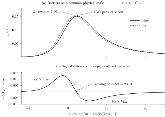
Quadrupolar Schwarzschild barriers for $m=GM$, $\ell=2$, and $C=0$. The upper panel uses a common $m^2V$ scale; the lower panel uses its own labeled $m^2(V_{\mathrm Z}-V_{\mathrm{RW}})$ scale. The polar peak lies at smaller $r_*/m$; the curves cross once outside the horizon. Both vanish toward the two asymptotic ends, which lie beyond this finite window. These quantitative curves do not by themselves prove isospectrality.

The numerical locations and heights are:

Feature	$r/m$	$r_*/m$	$m^2V$
Zerilli maximum	3.098791	1.900917	0.151310606
Regge–Wheeler maximum	3.280776	2.389415	0.151286700
Shared value at the crossing	3.190339	2.152521	0.151003119

The peak heights differ by only about $0.016\%$. The lower panel compares the two potentials at the same $r_*$, not their independently located maxima. The quadrupolar-barrier exercise derives their exact difference and crossing. The boundary-preserving transformation developed below, not visual similarity, explains their conditional spectral equivalence.

Horizon regularity should be checked in a regular chart, not inferred from a singular Schwarzschild time coordinate. With $v=t+r_*$,

$$\Box_2 =2\partial_v\partial_r+f\partial_r^2+f'\partial_r,$$

and (5) is finite at $r=2m$. Thus $(\Box_2-U_{\mathrm Z})\Psi=0$ is manifestly regular at the future horizon.

Boundary waves and exceptional multipoles

With the inherited Fourier convention $\Psi(t,r)=e^{-i\omega t}\psi(r)$, the future-horizon ingoing wave and the future-null-infinity outgoing wave are

$$e^{-i\omega(t+r_*)}=e^{-i\omega v}, \qquad e^{-i\omega(t-r_*)}=e^{-i\omega u},$$

respectively. Here $v=t+r_*$ is advanced time and $u=t-r_*$ is retarded time. The signs name causal propagation toward the two future boundaries; they are not interchangeable conventions for the radial exponential.

The derivation above cannot be analytically continued to the low multipoles. At $\ell=0$, the even vector harmonic and trace-free tensor harmonic vanish, but the scalar angular trace $\Omega_{AB}Y^{00}$ survives. A vacuum monopole that is regular at the future horizon and asymptotically flat changes the Schwarzschild mass, modulo gauge and after fixing the normalization of asymptotic time. At $\ell=1$, $Y_{AB}^{1m}$ vanishes. A regular vacuum even dipole has no radiative invariant: once the asymptotic origin is fixed it is pure gauge; if asymptotic translations are retained, it records a change of center-of-mass frame.

Neither conclusion follows by inserting $\lambda=-1$ or $0$ into (6), because the harmonic basis and constraint rank used to derive that equation have already changed. See Low Multipoles, Parameter Shifts, and Gauge Modes for the direct solutions and Martel and Poisson 2005, § VIII.A and § VIII.C, pp. 10–12 for the covariant equations.

An independent axial–polar check

The complicated rational coefficients in (6) admit a stringent check against the much simpler Regge–Wheeler equation. Define

$$\begin{aligned} \alpha&=\frac{\lambda(\lambda+1)}{3m}, &W(r)&=\alpha+\frac{3mf}{r(\lambda r+3m)},\\ D&=\frac{d}{dr_*}=f\frac{d}{dr}. \end{aligned}$$

Direct differentiation gives the two exact identities

$$V_{\mathrm{RW}}=W^2-DW-\alpha^2, \qquad V_{\mathrm Z}=W^2+DW-\alpha^2. \tag{9}$$

Let $A=D+W$. Its formal adjoint with respect to $dr_*$ is $A^\dagger=-D+W$; this dagger is not the Hilbert-space adjoint on a quasinormal-mode domain, whose outgoing boundary conditions are non-self-adjoint. Define the radial operators

$$H_{\mathrm{RW}}=-D^2+V_{\mathrm{RW}}, \qquad H_{\mathrm Z}=-D^2+V_{\mathrm Z}.$$

Equation (9) implies

$$H_{\mathrm{RW}}=A^\dagger A-\alpha^2, \qquad H_{\mathrm Z}=AA^\dagger-\alpha^2, \qquad AH_{\mathrm{RW}}=H_{\mathrm Z}A.$$

Therefore, if $H_{\mathrm{RW}}\psi_{\mathrm{RW}}=\omega^2\psi_{\mathrm{RW}}$, then the explicitly transformed field

$$\widehat\psi_{\mathrm Z}=A\psi_{\mathrm{RW}}$$

satisfies $H_{\mathrm Z}\widehat\psi_{\mathrm Z}=\omega^2\widehat\psi_{\mathrm Z}$. This verifies the entire potential, not only one limiting coefficient.

At both tortoise endpoints $W\to\alpha$, giving the endpoint multipliers

$$A e^{-i\omega r_*}\sim(\alpha-i\omega)e^{-i\omega r_*} \quad (\mathcal H^+),$$ $$A e^{+i\omega r_*}\sim(\alpha+i\omega)e^{+i\omega r_*} \quad (\mathscr I^+).$$

For complex frequency, these formulas refer to retarded endpoint solutions first selected where $\operatorname{Im}\omega>0$ and then analytically continued on a fixed sheet. A leading exponential alone does not select a quasinormal boundary solution at every frequency. The continued Jost-solution argument and its exceptional cases are developed on Chandrasekhar Transformations and Isospectrality.

For scattering at real $\omega>0$, $|\alpha-i\omega|=|\alpha+i\omega|=\sqrt{\alpha^2+\omega^2}$. The operator $A$ has dimensions of inverse length, so $A\psi_{\mathrm{RW}}$ is an unnormalized mathematical eigenfunction, not yet a physical Zerilli–Moncrief field. Its squared boundary amplitudes and derivatives acquire the dimensionful factor $\alpha^2+\omega^2$. For a radiation-adapted Cunningham–Price–Moncrief input, a horizon-normalized physical field is instead

$$\psi_{\mathrm{even}}^{(\mathcal H)} =\frac{(D+W)\psi_{\mathrm{odd}}}{\alpha-i\omega}. \tag{10}$$

It preserves an ingoing horizon amplitude, while an outgoing infinity amplitude acquires only $(\alpha+i\omega)/(\alpha-i\omega)$, a phase of unit modulus. Thus consistently normalized physical fluxes agree for real $\omega$. The map preserves wave type but does not preserve the raw numerical amplitude or even its physical dimension without this normalization.

The inverse contains $(\omega^2+\alpha^2)^{-1}$ and fails at the algebraically special frequency, including the damped choice $\omega=-i\alpha$. Equality of axial and polar spectra consequently requires the same vacuum Schwarzschild domain, the same horizon and infinity conditions, and an invertible map; it does not follow from the potentials looking similar. Chandrasekhar Transformations and Isospectrality develops the boundary-domain statement and exceptional solution in detail.

Radiation normalization and positive future flux

The master equation is linear, but radiated energy first appears at quadratic order in the small perturbation. We retain that leading order below. Sphere-harmonic indices in the norm are raised with the unit-sphere metric $\Omega^{AB}$:

$$\int_{S^2}\overline{Y}_{AB}^{\ell m}Y^{AB\ell' m'}\,d\Omega =\frac12\frac{(\ell+2)!}{(\ell-2)!} \delta_{\ell\ell'}\delta_{mm'}.$$

Suppose the material source is confined to a bounded region, so the neighborhood of future null infinity is vacuum. In outgoing coordinates, use the radiation gauge of Martel and Poisson, $t^ap_{ab}=t^ap_{aB}=0$, where $t^a=(\partial_u)^a$ is the Schwarzschild Killing vector normalized at infinity. This is a condition on contraction with a Killing vector, not a null-tetrad radiation-gauge definition. Their asymptotic vacuum equations give the even radiative metric

$$p_{AB}^{\mathrm{rad,even}} =r\sum_{\ell m}\Psi_{\mathrm{even}}^{\ell m}(u,\infty) Y_{AB}^{\ell m}+O(1).$$

The distinction between a coordinate metric component and physical strain is essential. On a sphere of radius $r$, the background metric and inverse are $q_{AB}=r^2\Omega_{AB}$ and $q^{AB}=r^{-2}\Omega^{AB}$. The transverse-traceless energy flux is

$$\left\langle\frac{dE_\infty^{\mathrm{even}}}{du}\right\rangle =\lim_{r\to\infty}\frac{r^2}{32\pi G} \int_{S^2} \left\langle \partial_up_{AB}^{\mathrm{rad,even}}\, \partial_up_{CD}^{\mathrm{rad,even}} \right\rangle q^{AC}q^{BD}\,d\Omega.$$

Each metric perturbation supplies one power of $r$, the two inverse sphere metrics supply $r^{-4}$, and the area supplies $r^2$. All radius factors cancel. Orthogonality then supplies the tensor norm, including its factor $1/2$, and gives

$$\left\langle\frac{dE_\infty^{\mathrm{even}}}{du}\right\rangle =\frac{1}{64\pi G} \sum_{\ell\geq2}\sum_{m=-\ell}^{\ell} \frac{(\ell+2)!}{(\ell-2)!} \left\langle \left|\partial_u\Psi_{\mathrm{even}}^{\ell m}(u,\infty)\right|^2 \right\rangle\geq0. \tag{11}$$

The brackets are the characteristic-time average used in the cited radiative formula. In the complex harmonic basis, a real perturbation obeys $\Psi^{\ell,-m}=(-1)^m\overline{\Psi^{\ell m}}$; the complete $m$ sum in (11) implements that reality condition rather than treating the paired modes as unrelated real fields. Do not take a second real part of each coefficient and then insert another universal factor $1/2$. For a single real $m=0$ sinusoid the usual time average of its squared derivative does give $1/2$; for a paired complex mode the two real angular quadratures are already included by the full sum.

If matter also stays out of an open neighborhood of the event horizon, a regular ingoing chart with $v=t+r_*$ permits the same Killing-vector conditions, now with $t^a=(\partial_v)^a$. Choose the horizon at $r_+=2m$ and angular labels comoving with its generators. In this gauge the radiative perturbation of the horizon’s intrinsic metric is

$$p_{AB}^{\mathcal H,\mathrm{even}} =r_+\sum_{\ell m}\Psi_{\mathrm{even}}^{\ell m}(v,r_+)Y_{AB}^{\ell m}.$$

Its first-order shear is $\sigma_{AB}=\tfrac12\partial_vp_{AB}^{\mathcal H,\mathrm{even}}$; indices in $\sigma_{AB}\sigma^{AB}$ are raised with the background horizon inverse metric $r_+^{-2}\Omega^{AB}$, twice. The horizon energy law comes from shear and area increase, not from applying the large-radius TT approximation at $r=2m$.

For a weak vacuum perturbation that settles between stationary eras, the leading Raychaudhuri equation for the area expansion $\vartheta$ is

$$\partial_v\vartheta=\kappa\vartheta-\sigma_{AB}\sigma^{AB}, \qquad \kappa=\frac{1}{4m}.$$

Vanishing expansion at the endpoints removes its total derivative upon integration. Equivalently, an average on times long compared with $\kappa^{-1}$ neglects the endpoint transient. With settled endpoints the perturbative first law is explicitly

$$\Delta E_{\mathcal H} =\frac{\kappa\,\Delta A}{8\pi G} =\frac{1}{8\pi G}\int dv\int_{\mathcal H_v} \sigma_{AB}\sigma^{AB}\,dA.$$

Its averaged rate is

$$\left\langle\frac{dE_{\mathcal H}^{\mathrm{even}}}{dv}\right\rangle =\frac{1}{8\pi G}\int_{\mathcal H_v} \left\langle\sigma_{AB}\sigma^{AB}\right\rangle\,dA, \qquad dA=r_+^2\,d\Omega.$$

The two factors of $1/2$ from the shears supply $1/4$, and the radius factors cancel as at infinity. Thus the same positive coefficient describes energy entering the Schwarzschild hole:

$$\left\langle\frac{dE_{\mathcal H}^{\mathrm{even}}}{dv}\right\rangle =\frac{1}{64\pi G} \sum_{\ell\geq2}\sum_{m=-\ell}^{\ell} \frac{(\ell+2)!}{(\ell-2)!} \left\langle \left|\partial_v\Psi_{\mathrm{even}}^{\ell m}(v,2m)\right|^2 \right\rangle\geq0. \tag{12}$$

This is an averaged absorption rate or an accumulated energy change with settled endpoints, not a definition-independent instantaneous mass derivative on an arbitrary horizon cut. The total change must remain small compared with $M$. No slow-motion or low-frequency restriction on the individual Schwarzschild modes is introduced by this calculation.

Equation (11) and its metric normalization follow from Martel and Poisson 2005, § VI, pp. 8–9, eqs. (6.2)–(6.8) and (6.16), PDF; the horizon metric and (12) are Martel and Poisson 2005, § VII, pp. 9–10, eqs. (7.1)–(7.5), PDF. The horizon gauge, shear law and averaging assumptions are developed in Poisson 2004, § IV, pp. 10–12, and § VI.A, pp. 17–18, PDF. The odd Cunningham–Price–Moncrief field carries the same coefficient. That agreement, together with the Darboux calculation above, checks the parity and normalization dictionaries independently.

What the scalar equation does and does not supply

Every regular vacuum even metric perturbation with $\ell\geq2$ produces a solution of the Zerilli equation. Conversely, any smooth local vacuum master solution reconstructs invariant metric data satisfying the Einstein constraints, as shown in Even-Parity Metric Perturbations. Constraint compatibility restricts independently specified metric initial data; it is not an additional constraint on the two master Cauchy-data functions. A global reconstruction still requires the chosen horizon and asymptotic conditions and an admissible gauge representative. Moncrief Invariants and Hamiltonian Reduction explains the reduced phase space, while Metric Reconstruction and Radiative Observables supplies the metric dictionary.

Smooth matter produces a smooth right-hand side. Point particles and thin shells can additionally produce delta and delta-prime terms, in which case the master field and its derivatives obey jump conditions. Those cases belong to Sourced Master Equations and Junction Conditions. Spectral solution methods remain in the response chapters, and generic numerical implementation belongs to Computational Relativity.

Common pitfalls

Confusing $\lambda$ with $\Lambda(r)$. The first is the constant $(\ell-1)(\ell+2)/2$; the second contains $6m/r$. Dropping that radial term destroys both the first-derivative cancellation and the potential.

Substituting exceptional multipoles into a radiative formula. The tensor basis and constraint rank change at $\ell=0,1$. Solve those sectors directly.

Equating Darboux-related potentials. $V_{\mathrm{RW}}$ and $V_{\mathrm Z}$ are different functions. Their conditional spectral relation follows from an intertwining operator plus boundary-domain information.

Comparing amplitudes before normalizations. A constant master-field rescaling leaves the homogeneous potential unchanged but changes the physical flux coefficient by the inverse square. A differential transform adds the boundary factors $\alpha\pm i\omega$ as well.

Exercises

Eliminate the polar constraint

Starting from (1) and (2), eliminate $\widetilde K$ and derive (3). Then use (1) and $Z_a=\nabla_a\zeta$ to prove the normalization relation (4).

Solution

Equation (2) gives

$$\widetilde K =-\frac{r}{\mu}\Box_2\zeta -\frac{2}{\mu}r^a\nabla_a\zeta.$$

Insert this in (1) and multiply by $\mu/r^2$. The coefficient of $r^a\nabla_a\zeta$ is

$$\frac{2\mu}{r}-\frac{2\Lambda}{r} =-\frac{2(\Lambda-\mu)}{r} =-\frac{12m}{r^2}.$$

The other two terms are $-\Lambda\Box_2\zeta$ and $L\mu\zeta/r^2$, which proves (3). Since $r^aZ_a=r^a\nabla_a\zeta$, divide (1) by $r\Lambda$:

$$\widetilde K+\frac{2}{\Lambda}r^aZ_a =-\frac{L}{r\Lambda}\zeta.$$

Multiplication by $2r/L$ gives $\Psi_{\mathrm{even}}=-2\zeta/\Lambda$ exactly.

Compare the quadrupolar barriers

Set $\ell=2$. Derive (8), expand both the Zerilli and Regge–Wheeler potentials through order $r^{-4}$, and find their nonhorizon crossing in the exterior.

Solution

Here $L=6$ and $\lambda=2$. Direct substitution in (6) gives

$$V_{\mathrm Z}^{\ell=2} =\frac{6f(4r^3+4mr^2+6m^2r+3m^3)} {r^3(2r+3m)^2}.$$

Expansion at large $r$ yields

$$V_{\mathrm Z}^{\ell=2} =\frac6{r^2}-\frac{24m}{r^3} +\frac{111m^2}{2r^4}+O(r^{-5}),$$

whereas

$$V_{\mathrm{RW}}^{\ell=2} =f\left(\frac6{r^2}-\frac{6m}{r^3}\right) =\frac6{r^2}-\frac{18m}{r^3} +\frac{12m^2}{r^4}.$$

Their exact difference factors as

$$V_{\mathrm Z}^{\ell=2}-V_{\mathrm{RW}}^{\ell=2} =-\frac{6m(r-2m)(4r^2-9mr-12m^2)} {r^4(2r+3m)^2}.$$

Besides the shared horizon zero, the positive root is

$$\frac{r}{m}=\frac{9+\sqrt{273}}{8}\simeq3.19034.$$

Both barriers are positive outside $r=2m$, but they are not identical: the Zerilli barrier lies above the Regge–Wheeler barrier just outside the horizon and below it beyond this crossing.

Normalize a transformed scattering solution

Let a Regge–Wheeler solution at real $\omega>0$, incident from infinity, have

$$\begin{aligned} \psi_{\mathrm{odd}}&\sim e^{-i\omega r_*}+\mathcal R_{\mathrm{odd}}e^{+i\omega r_*} && (r_*\to+\infty),\\ \psi_{\mathrm{odd}}&\sim \mathcal T_{\mathrm{odd}}e^{-i\omega r_*} && (r_*\to-\infty). \end{aligned}$$

Use (10) to find the polar reflection and transmission amplitudes. Show that their flux magnitudes agree with the axial ones, and explain why the same normalization cannot be used at $\omega=-i\alpha$.

Solution

At infinity, $D+W$ multiplies the incoming wave by $\alpha-i\omega$ and the outgoing wave by $\alpha+i\omega$. Division by $\alpha-i\omega$ therefore retains unit incident amplitude and gives

$$\mathcal R_{\mathrm{even}} =\frac{\alpha+i\omega}{\alpha-i\omega}\mathcal R_{\mathrm{odd}}.$$

The transmitted horizon wave has the same $e^{-i\omega r_*}$ orientation and the same multiplier as the incident wave, so

$$\mathcal T_{\mathrm{even}}=\mathcal T_{\mathrm{odd}}.$$

For real $\omega$, the ratio multiplying $\mathcal R$ has unit modulus. Therefore $|\mathcal R_{\mathrm{even}}|^2=|\mathcal R_{\mathrm{odd}}|^2$ and $|\mathcal T_{\mathrm{even}}|^2=|\mathcal T_{\mathrm{odd}}|^2$; with the common radiation-adapted coefficient, the reflected and transmitted physical fluxes agree. At $\omega=-i\alpha$, the denominator vanishes. That is the algebraically special obstruction, not a legitimate scattering normalization.

Count the energy of a real quadrupolar pulse

At future null infinity, let the only nonzero coefficients be

$$\Psi_{\mathrm{even}}^{22} =a\,e^{-u^2/(2\tau^2)}e^{-i\omega u}, \qquad \Psi_{\mathrm{even}}^{2,-2} =\overline{\Psi_{\mathrm{even}}^{22}},$$

with real $a$, $\tau>0$ and real $\omega$. This specifies a real angular perturbation; $a$ and $\tau$ have length dimension. Compute the quadratic radiative power underlying (11) and its whole-pulse integral. Identify the errors made by omitting the negative-$m$ partner, inserting an extra factor $1/2$, or differentiating only the carrier phase. This is a boundary-profile normalization problem, not a claim that scattering produces the same pulse at both boundaries.

Solution

For each member of the pair,

$$\left|\partial_u\Psi_{\mathrm{even}}^{22}\right|^2 =a^2e^{-u^2/\tau^2} \left(\omega^2+\frac{u^2}{\tau^4}\right).$$

The cross term vanishes because the envelope derivative is real and the phase derivative is imaginary. For $\ell=2$, the factorial ratio in (11) is $24$, and there are two equal mode contributions. Hence

$$P(u)=\frac{3a^2}{4\pi G}e^{-u^2/\tau^2} \left(\omega^2+\frac{u^2}{\tau^4}\right).$$

The real and imaginary parts of $\Psi^{22}$ multiply two orthogonal real angular patterns. Their squared derivatives add, so no second sinusoidal factor $1/2$ is needed. The Gaussian integrals

$$\int_{-\infty}^{\infty}e^{-u^2/\tau^2}\,du=\sqrt{\pi}\tau, \qquad \int_{-\infty}^{\infty}u^2e^{-u^2/\tau^2}\,du =\frac{\sqrt{\pi}}{2}\tau^3$$

give the whole-pulse energy

$$E_\infty=\int_{-\infty}^{\infty}P(u)\,du =\frac{3a^2}{4\sqrt{\pi}G} \left(\omega^2\tau+\frac{1}{2\tau}\right).$$

A fixed normalized convolution time average preserves this whole-time integral. Omitting the partner or adding an extra $1/2$ halves the energy. Omitting the envelope derivative removes the $1/(2\tau)$ term; even at $\omega=0$ the time-varying envelope radiates. The result has dimension length$/G$, as required for energy in the units used here.

References

• Martel, K., and Poisson, E. (2005). “Gravitational perturbations of the Schwarzschild spacetime: A practical covariant and gauge-invariant formalism.” Physical Review D 71, 104003. DOI. Open PDF.
• Poisson, E. (2004). “Absorption of mass and angular momentum by a black hole: Time-domain formalisms for gravitational perturbations, and the small-hole/slow-motion approximation.” Physical Review D 70, 084044. DOI. Open PDF.
• Sarbach, O., and Tiglio, M. (2001). “Gauge-invariant perturbations of Schwarzschild black holes in horizon-penetrating coordinates.” Physical Review D 64, 084016. DOI. Open PDF.
• Zerilli, F. J. (1970). “Effective potential for even-parity Regge–Wheeler gravitational perturbation equations.” Physical Review Letters 24, 737–738. DOI.
• Zerilli, F. J. (1970). “Gravitational field of a particle falling in a Schwarzschild geometry analyzed in tensor harmonics.” Physical Review D 2, 2141–2160. DOI.