Bäcklund and Related Transformations

A Bäcklund transformation is a first-order bridge between two solutions of a nonlinear field equation. For stationary-axisymmetric vacuum gravity, that bridge can be encoded as a polynomial transformation of the Ernst linear system. This page develops the construction far enough to turn a Minkowski seed into the exact subextremal Kerr metric, then asks the essential physical question: did the map create a new spacetime, or merely rename the seed?

Required background. Killing Fields and Isometry Groups supplies the stationary and axial symmetry reduction.

Helpful background. Einstein’s Equation supplies the vacuum equations; The Riemann Curvature Tensor supplies invariant comparison; Exact Solutions of Einstein’s Equations supplies Minkowski, Schwarzschild, and Kerr benchmarks; Formulations of General Relativity supplies reduced field equations; PDEs and Green Functions supplies compatibility and boundary data.

The gravitational construction assumes four-dimensional, stationary-axisymmetric, Ricci-flat vacuum with $\Lambda=0$. It is local on a connected Weyl patch. Twist and Ernst Potentials and Weyl–Papapetrou Form and Orbit Space supply the reduction and reconstruction used below.

A first-order bridge between Ernst fields

Let $\xi=\partial_t$ be the stationary Killing field and $\eta=\partial_\varphi$ the axial Killing field, with $\varphi\sim\varphi+2\pi$. In a region where $\xi$ is timelike, set

$$f=-\xi^\mu\xi_\mu>0, \qquad \omega_\mu=\epsilon_{\mu\nu\rho\sigma} \xi^\nu\nabla^\rho\xi^\sigma, \qquad d\chi=\omega,$$

and choose the additive twist gauge so that $\chi\to0$ at the selected asymptotically flat end. With the site orientation $\epsilon_{tr\theta\varphi}=+\sqrt{-g}$, the Ernst potential is

$$\mathcal E=f+i\chi.$$

In Weyl coordinates $(\rho,z)$ it obeys

$$(\operatorname{Re}\mathcal E) \left(\mathcal E_{,\rho\rho}+\rho^{-1}\mathcal E_{,\rho} +\mathcal E_{,zz}\right) =\mathcal E_{,\rho}^2+\mathcal E_{,z}^2.$$

A differential Bäcklund transformation writes first-order equations coupling a seed $\mathcal E_0$ to an output $\mathcal E_1$. Its cross-derivative condition must be the seed Ernst equation, and the same identities must imply the output Ernst equation. That compatibility is the solution-generating theorem. Reality, asymptotic normalization, and axis regularity are additional conditions; compatibility alone does not impose them.

The table fixes the convention-sensitive data before the transformation is written.

Object	Convention used here	Why it matters
Metric and orientation	Signature $(-,+,+,+)$ and $\epsilon_{tr\theta\varphi}=+\sqrt{-g}$	Fixes the signs of $f$, $\chi$, and the Kerr angular momentum.
Weyl base	$\rho\ge0$ with orientation $d\rho\wedge dz$	Fixes the ordering of the two first-order equations and the horizon rod orientation.
Complex coordinate	$\zeta=\rho+iz$	Separates the constant spectral datum $K$ from the coordinate-dependent square root $\Lambda$.
Ernst gauge	$\mathcal E\to1$ and $\chi\to0$ at the chosen infinity	Removes time normalization and additive twist ambiguities.
Reality sector	Real $K$ with unit-modulus auxiliary data, or conjugate-paired $K$ and auxiliary data	Makes the reconstructed metric real.

A transparent compatibility example

Before introducing the matrix construction, it helps to see the same cross-derivative logic in a scalar equation. Let a seed $u$ and a candidate $v$ be coupled in light-cone coordinates $(x_+,x_-)$, and define

$$P=\frac{v+u}{2}, \qquad Q=\frac{v-u}{2}.$$

For a real parameter $\kappa\ne0$, impose the first-order pair

$$P_{,+}=\kappa\sin Q, \qquad Q_{,-}=\kappa^{-1}\sin P.$$

Cross-differentiation gives

$$\frac{v_{,+-}+u_{,+-}}2=\sin P\cos Q, \qquad \frac{v_{,+-}-u_{,+-}}2=\sin Q\cos P.$$

Adding and subtracting these equations yields

$$v_{,+-}=\sin(P+Q)=\sin v, \qquad u_{,+-}=\sin(P-Q)=\sin u.$$

Thus the seed sine–Gordon equation is exactly the path-independence condition for constructing $v$, and the output satisfies the same nonlinear equation. Reversing only one sign in the first-order pair instead generates the opposite sign of the sine–Gordon equation. This convention is equivalent to the classical auto-Bäcklund pair developed in Rogers and Shadwick 1982, §1.2, pp. 16–21.

The Ernst construction implements this same idea in matrix form: its auxiliary linear problem is overdetermined, and compatibility is precisely the nonlinear field equation.

The Neugebauer polynomial construction

Introduce a constant complex spectral datum $K$ and the coordinate-dependent quantity

$$\Lambda(K;\rho,z) =\sqrt{\frac{K-i\bar\zeta}{K+i\zeta}}.$$

The square-root sheet is chosen continuously on the working Weyl patch and normalized by $\Lambda\to1$ as $K\to\infty$. Thus $K$ is constant while $\Lambda$ is not. Confusing these two objects destroys the compatibility calculation.

We use the Wirtinger derivatives

$$\partial_\zeta=\frac12(\partial_\rho-i\partial_z), \qquad \partial_{\bar\zeta}=\frac12(\partial_\rho+i\partial_z).$$

For a seed $\mathcal E_0$ with $f_0=\operatorname{Re}\mathcal E_0$, define

$$M_0^3=\frac{\mathcal E_{0,\zeta}}{2f_0}, \quad M_0^4=\frac{\bar{\mathcal E}_{0,\zeta}}{2f_0}, \quad M_0^{*3}=\frac{\mathcal E_{0,\bar\zeta}}{2f_0}, \quad M_0^{*4}=\frac{\bar{\mathcal E}_{0,\bar\zeta}}{2f_0}.$$

Here the star is part of the traditional label for the $d\bar\zeta$ coefficients; complex conjugation is still shown by an overbar. Keeping that distinction visible prevents a common mistake when the seed is genuinely complex.

Its wavefunction $\Phi_0(\Lambda)$ solves

$$d\Phi_0= \left[ \begin{pmatrix} M_0^4&\Lambda M_0^4\\ \Lambda M_0^3&M_0^3 \end{pmatrix}d\zeta + \begin{pmatrix} M_0^{*4}&\Lambda^{-1}M_0^{*4}\\ \Lambda^{-1}M_0^{*3}&M_0^{*3} \end{pmatrix}d\bar\zeta \right]\Phi_0,$$

with the Ernst normalization

$$\Phi_0(1)= \begin{pmatrix} \bar{\mathcal E}_0&1\\ \mathcal E_0&-1 \end{pmatrix}.$$

The zero-curvature condition for this linear system is exactly the Ernst equation. Neugebauer’s transformation seeks a new wavefunction in the polynomial form

$$\Phi=q(\Lambda)P(\Lambda)\Phi_0, \qquad P(\Lambda)=\sum_{s=0}^{n}P_s\Lambda^s.$$

At every selected zero $\Lambda_k=\Lambda(K_k)$ of $\det P$, choose a constant nonzero projective vector $p^{(k)}$ and impose

$$P(\Lambda_k)\Phi_0(\Lambda_k)p^{(k)}=0.$$

Only the projective class matters: $p^{(k)}\sim c_kp^{(k)}$ for every nonzero constant $c_k$. After imposing the Ernst reduction’s spectral and parity structure on $P$, a matrix normalization such as $P(-1)=I$ leaves the kernel equations to determine the allowed independent coefficients algebraically. Without those reduction conditions, arbitrary $2\times2$ coefficients would be underdetermined by the kernel vectors alone. The scalar $q$ is fixed by

$$q_{,\bar\zeta}=0, \qquad (\Lambda^nq)_{,\zeta}=0,$$

so that the transformed connection retains the required trace and spectral normalization. The kernel conditions cancel the apparent poles of $P^{-1}$, so

$$\mathcal A =d(qP)(qP)^{-1}+(qP)\mathcal A_0(qP)^{-1}$$

has the same spectral form as the seed connection. Its curvature is

$$d\mathcal A-\mathcal A\wedge\mathcal A =(qP) \left(d\mathcal A_0-\mathcal A_0\wedge\mathcal A_0\right) (qP)^{-1}.$$

Hence a compatible seed produces a compatible output wherever the dressing matrix is nonsingular. The new Ernst field is read from $\Phi(1)$ in the same normalization. This is the precise version of “compatibility maps solutions to solutions”; the polynomial and kernel data make it executable. The construction and pole-cancellation argument are developed in Stephani et al. 2003, §10.6, pp. 146–148, and §34.4, pp. 538–541.

There is an equivalent first-order description. Set

$$\begin{pmatrix}l_k\\m_k\end{pmatrix} =\Phi_0(\Lambda_k)p^{(k)}, \qquad \alpha_k=\frac{l_k}{m_k}.$$

Then each auxiliary ratio obeys the Riccati system

$$\begin{aligned} d\alpha_k={}& \left[(\alpha_k+\Lambda_k)M_0^4 -\alpha_k(1+\Lambda_k\alpha_k)M_0^3\right]d\zeta\\ &+\left[(\alpha_k+\Lambda_k^{-1})M_0^{*4} -\alpha_k(1+\Lambda_k^{-1}\alpha_k)M_0^{*3}\right]d\bar\zeta. \end{aligned}$$

This formula follows directly by differentiating $\alpha_k=l_k/m_k$. For example,

$$l_{k,\zeta}=M_0^4(l_k+\Lambda_km_k), \qquad m_{k,\zeta}=M_0^3(\Lambda_kl_k+m_k).$$

There is a source-level pitfall here. Equation (34.93) of Stephani et al. prints a factorized $M_0^3$ term that is inconsistent with their preceding Eqs. (34.79) and (34.87). The displayed equation above is the quotient derived from those preceding equations; its quadratic-$\alpha_k$ structure is independently visible, after translating the spectral square-root convention, in Abdolrahimi, Kunz, and Nedkova 2015, §3, Eq. (19), pp. 8–9 (PDF).

For a real pole location $K_k$, the physical reality condition is $\alpha_k\bar\alpha_k=1$. Complex pole locations must occur in conjugate pairs with the corresponding cross-pairing of their $\alpha$ data. These conditions make the local field real; they do not remove NUT charge, conical defects, or zeros of the reconstruction denominator. Neugebauer’s original transformations and their recursive algebraization are given in Neugebauer 1979, pp. L67–L70 and Neugebauer 1980, pp. 1737–1740.

Permutability and the second generation

Neugebauer permutability is not ordinary commutativity with fixed parameters. In the Rogers–Shadwick convention, the two elementary transformations $I_1$ and $I_2$ use pseudopotentials $(\alpha_{\rm RS},\gamma_{\rm RS})$. These are not the projective wavefunction ratios $\alpha_k=l_k/m_k$ above; relating the two descriptions requires a convention-dependent Möbius and spectral dictionary.

For compactness, omit the subscript ${\rm RS}$ inside the following transport display only. The exact alternating $I_1/I_2$ loop closes with the transported parameters

$$\begin{aligned} \alpha'&=\frac{\alpha-\gamma}{\gamma(\alpha-1)}, &\gamma'&=\gamma^{-1},\\ \alpha''&=\frac{\gamma}{\alpha}, &\gamma''&=\gamma,\\ \alpha'''&=\frac{\alpha-1}{\alpha-\gamma}, &\gamma'''&=\gamma^{-1}. \end{aligned}$$

Now solve the two first-generation auxiliary systems once, using distinct data $(\alpha_{\mathrm{RS},1},\gamma_{\mathrm{RS},1})$ and $(\alpha_{\mathrm{RS},2},\gamma_{\mathrm{RS},2})$ on the same seed. Write $\mathcal X_0=(M_i,N_i)$ for the seed fields and $\mathcal X_A=I_1(\alpha_{\mathrm{RS},A},\gamma_{\mathrm{RS},A})\mathcal X_0$ for the two first-generation fields. The two data sets jointly determine the displayed second-generation parameter pair algebraically:

$$\alpha_{\mathrm{RS}}^{(2)} =\frac{\gamma_{\mathrm{RS},1}\alpha_{\mathrm{RS},2} -\alpha_{\mathrm{RS},1}\gamma_{\mathrm{RS},2}} {\gamma_{\mathrm{RS},1} (\alpha_{\mathrm{RS},2}-\alpha_{\mathrm{RS},1})}, \qquad \gamma_{\mathrm{RS}}^{(2)} =\frac{\gamma_{\mathrm{RS},2}^{2}}{\gamma_{\mathrm{RS},1}}.$$

These parameters enter the source’s displayed route

$$\mathcal X^{(2)} =I_2\!\left(\alpha_{\mathrm{RS}}^{(2)}, \gamma_{\mathrm{RS}}^{(2)}\right)\mathcal X_1.$$

No further Riccati integration is required. Both first-generation data sets enter the rational pair, but Eq. (1.564) does not justify obtaining a second route by merely swapping the labels $1\leftrightarrow2$ in that pair. The four-step loop above is on the chart

$$\alpha_{\mathrm{RS}}\gamma_{\mathrm{RS}} (\alpha_{\mathrm{RS}}-1) (\alpha_{\mathrm{RS}}-\gamma_{\mathrm{RS}})\ne0.$$

For the displayed second-generation route, the full chart condition is

$$\begin{aligned} \alpha_{\mathrm{RS},1}\alpha_{\mathrm{RS},2} \gamma_{\mathrm{RS},1}\gamma_{\mathrm{RS},2}&\ne0,\\ \alpha_{\mathrm{RS},2}-\alpha_{\mathrm{RS},1}&\ne0, &\gamma_{\mathrm{RS},1}\alpha_{\mathrm{RS},2} -\alpha_{\mathrm{RS},1}\gamma_{\mathrm{RS},2}&\ne0. \end{aligned}$$

The final factor is the numerator of $\alpha_{\mathrm{RS}}^{(2)}$; if it vanished, the last $I_2$ input would leave this chart. If any displayed factor vanishes, cancellation through the formula is not valid: the case needs a separate chart or limiting calculation. Complex intermediate fields also require the stated reality pairing. Rogers and Shadwick 1982, §1.19, Theorem 1.13 and Eqs. (1.561)–(1.564), pp. 118–120 proves the exact parameter transport and construction.

The figure makes the two input branches and their joint parameter map visible. Read the dashed box separately: the theorem produces a local reduced-system solution, not yet a real, regular, asymptotically normalized spacetime.

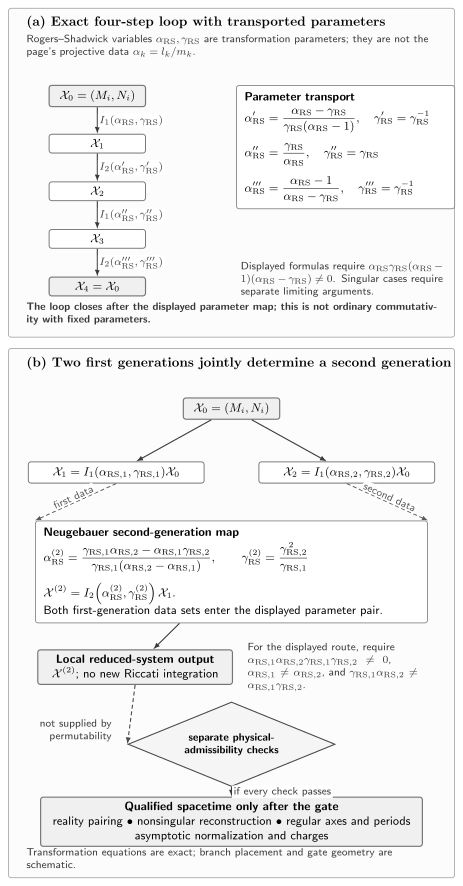
Neugebauer permutability is not ordinary commutativity with fixed parameters. The upper composition closes only after the displayed $I_1/I_2$ parameter map. For two first-generation data sets, $\alpha_{\mathrm{RS}}^{(2)}=(\gamma_{\mathrm{RS},1}\alpha_{\mathrm{RS},2}-\alpha_{\mathrm{RS},1}\gamma_{\mathrm{RS},2})/[\gamma_{\mathrm{RS},1}(\alpha_{\mathrm{RS},2}-\alpha_{\mathrm{RS},1})]$ and $\gamma_{\mathrm{RS}}^{(2)}=\gamma_{\mathrm{RS},2}^{2}/\gamma_{\mathrm{RS},1}$, so the second generation is obtained algebraically with no new Riccati integration. The equations are exact and the layout is schematic. Reality, nonsingular reconstruction, axis regularity, and asymptotic normalization require separate checks.

Minkowski to Kerr: a complete benchmark

Take the asymptotically normalized flat Weyl seed

$$ds_0^2=-dt^2+d\rho^2+dz^2+\rho^2d\varphi^2, \qquad \mathcal E_0=1, \qquad A_{\varphi,0}=k_0=0,$$

with $\varphi\sim\varphi+2\pi$. Apply two distinct sets of Neugebauer data to this same seed. They produce two first-generation branches whose data jointly fix the displayed second-generation output algebraically. Reality, asymptotic normalization, and zero NUT charge are imposed on that output, not on either first-generation branch in isolation.

In the Rogers–Shadwick flat-seed solution, $b_1$ and $b_2$ are integration constants for the two first-generation pseudopotential systems. They should not be identified directly with the projective ratios $\alpha_k$ without the missing convention dictionary. The zero-NUT subextremal slice can be parametrized by

$$b_1=e^{2i\beta}, \qquad b_2=-e^{i\beta}, \qquad K_1=z_0-\sigma, \qquad K_2=z_0+\sigma,$$

where

$$m>0, \qquad -\frac{\pi}{2}<\beta<\frac{\pi}{2}, \qquad a=m\sin\beta, \qquad \sigma=m\cos\beta=\sqrt{m^2-a^2}>0.$$

The physical parameter count is transparent. The length $m$ becomes the mass parameter, $a/m=\sin\beta$ is the dimensionless rotation, and $\sigma$ is derived rather than independent. The midpoint $z_0=(K_1+K_2)/2$ is removable by translating the Weyl $z$ origin. The two branch points therefore contribute a separation $2\sigma$, not an additional location observable. The algebraic recombination gives

$$\mathcal E_{\rm B} =\frac{ e^{-i\beta}r_1+e^{i\beta}r_2-2m\cos\beta }{ e^{-i\beta}r_1+e^{i\beta}r_2+2m\cos\beta }, \qquad r_A=\sqrt{\rho^2+(z-K_A)^2}.$$

Geometrically, $r_A$ is the ordinary Euclidean distance in the auxiliary $(\rho,z)$ half-plane from the field point to the marked axis point $K_A$. The two distances are natural variables for the finite interval between $K_1$ and $K_2$; prolate coordinates simply replace their sum and difference by $x$ and $y$.

This is the zero-NUT specialization of the paired Minkowski output in Rogers and Shadwick 1982, §1.19, pp. 119–122, especially Eqs. (1.565)–(1.577). Setting the NUT parameter to zero before defining $a$ is important: the generic Kerr–NUT parameter dictionary is convention-sensitive, whereas this slice has horizon half-length $\sigma$, with $\sigma^2=m^2-a^2$.

Introduce prolate coordinates by

$$\rho=\sigma\sqrt{x^2-1}\sqrt{1-y^2}, \qquad z-z_0=\sigma xy,$$

so that

$$r_1=\sigma(x+y), \qquad r_2=\sigma(x-y), \qquad x=\frac{r_1+r_2}{2\sigma}, \qquad y=\frac{r_1-r_2}{2\sigma}.$$

The exterior prolate domain is

$$x\ge1, \qquad -1\le y\le1, \qquad r_1,r_2\ge0.$$

The segment $x=1$ is the finite interval $\rho=0$, $z_0-\sigma\le z\le z_0+\sigma$; its endpoints are the two branch points. The exterior axes are $y=+1$ and $y=-1$ away from that segment.

The Bäcklund output simplifies without approximation:

$$\mathcal E_{\rm B} =\frac{\sigma x-iay-m}{\sigma x-iay+m}.$$

Now make the bidirectional coordinate change

$$r=m+\sigma x, \qquad y=\cos\theta, \qquad \rho=\sqrt{\Delta}\sin\theta, \qquad z-z_0=(r-m)\cos\theta,$$

where

$$\Sigma=r^2+a^2\cos^2\theta, \qquad \Delta=r^2-2mr+a^2.$$

On the black-hole exterior this map has

$$r\ge r_+=m+\sigma, \qquad 0\le\theta\le\pi.$$

For $\sigma>0$ the formulas are invertible between the prolate exterior and this Boyer–Lindquist exterior, including their boundary intervals in the usual limiting sense.

Then

$$\mathcal E_{\rm B} =1-\frac{2m}{r-ia\cos\theta},$$

and therefore

$$f=1-\frac{2mr}{\Sigma}, \qquad \chi=-\frac{2ma\cos\theta}{\Sigma}.$$

The negative sign in $\chi$ follows from the stated spacetime orientation. The isometry $\varphi'=-\varphi$ rewrites the same metric with $a'=-a$ and sends the signed Komar charge $J[\partial_\varphi]$ to $J[\partial_{\varphi'}]=-J[\partial_\varphi]$. On the same oriented manifold, $\chi$ is a scalar and does not flip under this passive coordinate change. If the site component-orientation convention $\epsilon_{tr\theta\varphi'}=+\sqrt{-g}$ is reimposed in the primed chart, the printed twist potential changes sign as well; that comparison uses the orientation-reversed isometric representative, not a second physical family.

Reconstruction of the four-metric

Use the stationary ansatz

$$ds^2=-f(dt+A_\varphi d\varphi)^2 +f^{-1}\left[e^{2k}(d\rho^2+dz^2)+\rho^2d\varphi^2\right].$$

The first-order reconstruction equations, with constants fixed at infinity and on a regular axis, give

$$A_\varphi =\frac{2mar\sin^2\theta}{\Sigma-2mr}, \qquad e^{2k} =\frac{\Sigma-2mr} {(r-m)^2-\sigma^2\cos^2\theta}.$$

The reduction began on a patch where $\partial_t$ is timelike, so the individual timelike-reduction variables cease to be a regular chart at the stationary-limit surface $f=0$: $f^{-1}$ and $A_\varphi$ separately diverge there. This does not make the ergosurface a spacetime singularity. Their combinations in the reconstructed Boyer–Lindquist four-metric have an analytic continuation through $f=0$. Substitution yields

$$\begin{aligned} ds^2={}&-\left(1-\frac{2mr}{\Sigma}\right)dt^2 -\frac{4mar\sin^2\theta}{\Sigma}\,dt\,d\varphi +\frac{\Sigma}{\Delta}\,dr^2+\Sigma\,d\theta^2\\ &+\frac{\sin^2\theta}{\Sigma} \left[(r^2+a^2)^2-a^2\Delta\sin^2\theta\right]d\varphi^2, \end{aligned}$$

the Kerr metric in Boyer–Lindquist coordinates. This is stronger than recognizing a familiar Ernst numerator: it reconstructs every metric coefficient in the site convention.

Checks that distinguish a new spacetime

Several independent tests close the calculation.

• Reduced equation. In prolate coordinates the Ernst residual before imposing the endpoint relation is proportional to

  $$4m(iay+\sigma x)(a^2-m^2+\sigma^2).$$

  It vanishes exactly when $\sigma^2=m^2-a^2$.

• Unreduced equation. The reader-accessible SymPy checker constructs the Levi-Civita connection from the four-metric and evaluates all ten independent Ricci components at two exact subextremal points; every component vanishes. This exact-point regression complements the analytic identification with Kerr and avoids silently recycling the reduced equation. The Killing block also obeys

  $$g_{tt}g_{\varphi\varphi}-g_{t\varphi}^2 =-\Delta\sin^2\theta=-\rho^2,$$

  which also checks the canonical Weyl gauge.

• Signature. For $r>r_+=m+\sigma$ and $0<\theta<\pi$, the radial and polar entries are positive while the $t$–$\varphi$ block has negative determinant. It therefore has one negative and one positive eigenvalue even inside the ergoregion, where $g_{tt}$ changes sign.

• Charges. At large $r$,

  $$g_{tt}=-1+\frac{2m}{r}+O(r^{-2}), \qquad g_{t\varphi}=-\frac{2ma\sin^2\theta}{r}+O(r^{-2}).$$

  In geometric units, $M=m$ and $J=ma$; with $G$ restored, $M_{\rm ADM}=m/G$ and $J=ma/G$. Flat space has neither charge.

• Rods and axes. The outer horizon $r=r_+$ maps to the finite Weyl interval $\rho=0$, $z_0-\sigma\le z\le z_0+\sigma$. The two complementary intervals are regular axes when $\varphi$ has period $2\pi$ and the reconstruction constant is fixed as above.

• Limits. The limit $a\to0$ gives Schwarzschild. After reconstruction, taking $m\to0$ with $a/m$ fixed at a fixed Boyer–Lindquist or Weyl field point gives the complete Minkowski metric. The raw distinct-pole/prolate representation degenerates because $K_1,K_2\to z_0$, so it is not the chart in which to perform that limit. Likewise, $\lvert a\rvert\to m$ coalesces the branch points; extremal Kerr exists, but the distinct-pole and prolate formulas must be replaced by their controlled limit. The superextremal sector uses conjugate rather than distinct real branch points.

The map has therefore created a genuinely new geometry on the stated exterior, not a coordinate rewrite of Minkowski space. It produces nonzero curvature, ADM mass, angular momentum, and a finite horizon rod, with boundary and rod data unlike the seed. No claim about the maximal Kerr extension is needed for that conclusion.

New solution or reparametrized seed?

No single diagnostic answers every version of this question. Use the following hierarchy.

Test	What it can establish	Limitation
Potential gauge	A constant shift of $\chi$, or an allowed rescaling of the Killing generator before normalization, need not change the geometry.	A different printed $\mathcal E$ is not by itself evidence of a new spacetime.
Explicit isometry	A bidirectional coordinate and gauge map proves local equivalence on its stated domain.	It does not by itself compare global identifications or boundary normalization.
Cartan data	Different fully normalized Cartan invariants prove local inequivalence.	Scalar polynomial invariants alone may be incomplete.
Asymptotic charges	A new normalized mass, NUT charge, angular momentum, or electromagnetic charge proves inequivalence relative to the same asymptotic boundary data.	Charges require a specified end, normalization, and falloff class.
Global structure	Axis periods, horizons, asymptotic ends, and quotient identifications distinguish globally inequivalent spacetimes.	Locally identical quotients can still differ globally.

The scalar-invariant limitation is concrete. Minkowski space and the Ricci-flat plane wave

$$ds^2=-2\,du\,dv+dx^2+dy^2+(x^2-y^2)du^2$$

both have vanishing scalar polynomial curvature invariants. The wave is nevertheless not flat: its $R_{uxux}$ and $R_{uyuy}$ components are nonzero with opposite signs. The Cartan–Karlhede algorithm or an explicit frame comparison separates them; see Coley, Hervik, and Pelavas 2009, §§7–9, pp. 21–36. Conversely, a parameter that changes fully normalized Cartan data cannot be removed by a global coordinate identification. A parameter invisible locally may still distinguish global quotients after periods and boundary data are fixed.

The final physical checks—denominator zeros, signature, axes, horizons, charges, and global extensions—are developed systematically on Verifying and Interpreting Generated Solutions.

Relation to inverse scattering

The neighboring Inverse Scattering and Soliton Metrics page starts from a rational dressing matrix and reconstructs residues with a finite Gram system. Neugebauer’s construction starts from a polynomial wavefunction transformation or its Riccati variables. For this Ernst system, the two descriptions can be related, but only after matching their spectral coordinate, wavefunction normalization, reality involution, pole count, and determinant gauge; Omote and Wadati 1981, pp. 1621–1631 gives an explicit Ernst-specific comparison.

Feature	Neugebauer Bäcklund form	Rational inverse-scattering form
Auxiliary object	Polynomial $P(\Lambda)$ or Riccati ratios $\alpha_k$	Rational dressing matrix with simple spectral poles
Discrete data	Constants $K_k$ and projective kernel vectors	Pole locations and projective polarization vectors
Main finite calculation	Solve kernel equations for polynomial coefficients	Invert the finite Gram matrix of residues
Reality condition	Real or conjugate-paired $K_k$ with paired $\alpha_k$	Pole and residue data closed under the spectral involution
Normalization issue	Fix $P(-1)$, the trace factor $q$, and $\Phi(1)$	Repair the canonical determinant and fix the asymptotic Killing frame
Safe comparison	Match the final normalized Ernst field and reconstructed metric	Match the same field and metric, not a convention-dependent soliton label

Thus statements such as “one soliton is Kerr” are incomplete without a counting convention. The paired Neugebauer step above uses two real branch points; a different dressing convention may call the corresponding construction a soliton–antisoliton pair or a two-pole solution.

Iteration also separates local generation from global admissibility. A further paired transformation can produce the double-Kerr–NUT family as a local exact vacuum field, but that fact does not make it a regular equilibrium of two subextremal black holes. The axis conditions and horizon inequalities rule out that interpretation in the regular asymptotically flat two-horizon problem; see Neugebauer and Hennig 2009, §§2.4–4, pp. 2118–2127. This is precisely why the checks after reconstruction are part of the mathematics, not optional physical commentary.

Exercises

1. Generate the sine–Gordon kink

Starting from the seed $u=0$, derive every nonconstant solution of the displayed Bäcklund pair on the branch $0<v<2\pi$. Verify it directly in the second-order equation.

Solution

For $u=0$, $P=Q=v/2$, so

$$v_{,+}=2\kappa\sin\frac v2, \qquad v_{,-}=2\kappa^{-1}\sin\frac v2.$$

Because

$$\frac{d}{dv}\log\tan\frac v4 =\frac{1}{2\sin(v/2)},$$

the first equation gives $\log\tan(v/4)=\kappa x_++C(x_-)$. The second fixes $C'=\kappa^{-1}$, hence

$$v=4\arctan\exp \left(\kappa x_++\kappa^{-1}x_-+\delta\right).$$

Writing the exponent as $\Theta$, one finds $v_{,\Theta}=2\operatorname{sech}\Theta$ and $v_{,\Theta\Theta}=\sin v$. Since $\Theta_{,+}\Theta_{,-}=1$, $v_{,+-}=\sin v$.

2. Derive the projective Riccati equation

Let $(l,m)^{\mathsf T}$ solve the $d\zeta$ part of the displayed Lax system and set $\alpha=l/m$ on a patch where $m\ne0$. Derive $\alpha_{,\zeta}$. Then compare it with $(\alpha+\Lambda)(M^4-\alpha M^3)$ and find the difference.

Solution

The two matrix rows give

$$l_{,\zeta}=M^4(l+\Lambda m), \qquad m_{,\zeta}=M^3(\Lambda l+m).$$

The quotient rule therefore gives

$$\begin{aligned} \alpha_{,\zeta} &=\frac{l_{,\zeta}m-lm_{,\zeta}}{m^2}\\ &=(\alpha+\Lambda)M^4 -\alpha(1+\Lambda\alpha)M^3. \end{aligned}$$

Subtracting the factorized expression yields

$$\alpha(\alpha-1)(1-\Lambda)M^3,$$

which is not identically zero. Replacing $\Lambda$ by $\Lambda^{-1}$ and $M^j$ by $M^{*j}$ gives the $d\bar\zeta$ coefficient. This exercise is also a useful rule for source checking: a cited formula must remain compatible with the equations that define its variables.

3. Prove preservation of zero curvature

Let $D=qP$ be nonsingular away from its prescribed spectral points and define $\mathcal A=dD\,D^{-1}+D\mathcal A_0D^{-1}$. Show that the curvature of $\mathcal A$ is the conjugate of the seed curvature.

Solution

Set

$$B=dD\,D^{-1}, \qquad C=D\mathcal A_0D^{-1}, \qquad \mathcal A=B+C.$$

Using $d(D^{-1})=-D^{-1}(dD)D^{-1}$ gives

$$dB-B\wedge B=0, \qquad dC=B\wedge C+C\wedge B+D(d\mathcal A_0)D^{-1}.$$

Therefore

$$\begin{aligned} d\mathcal A-\mathcal A\wedge\mathcal A &=(dB-B\wedge B)\\ &\quad +(dC-B\wedge C-C\wedge B-C\wedge C)\\ &=D(d\mathcal A_0-\mathcal A_0\wedge\mathcal A_0)D^{-1}. \end{aligned}$$

Thus a flat seed connection remains flat. At a zero of $\det P$, nonsingularity is replaced by the kernel conditions: they cancel the apparent pole in the transformed connection before this identity is continued across the point.

4. Read the Kerr charges from the output

Starting from $\mathcal E=1-2m/(r-ia\cos\theta)$, derive $f$ and $\chi$ and read the leading mass and angular-momentum coefficients from the reconstructed metric.

Solution

Multiplying by the complex conjugate denominator gives

$$\mathcal E =1-\frac{2m(r+ia\cos\theta)}{\Sigma},$$

so

$$f=1-\frac{2mr}{\Sigma}, \qquad \chi=-\frac{2ma\cos\theta}{\Sigma}.$$

At large $r$, $g_{tt}=-1+2m/r+O(r^{-2})$ and $g_{t\varphi}=-2ma\sin^2\theta/r+O(r^{-2})$. The standard asymptotically flat normalization therefore gives $M=m$ and $J=ma$ in geometric units. Since the flat seed has $M=J=0$, these normalized charges cannot arise from a coordinate reparametrization of that seed.

5. Separate time normalization from new physics

In

$$ds^2=-f(dt+A)^2+f^{-1}h,$$

suppose the same noncompact Killing flow is relabeled by $t'=t/c$, with $c>0$ so time orientation is fixed. Determine the transformed reduced fields and explain when the change is pure reparametrization.

Solution

Since $t=ct'$,

$$dt+A=c\left(dt'+\frac{A}{c}\right).$$

The same four-metric has

$$f'=c^2f, \qquad A'=\frac{A}{c}, \qquad h'=c^2h, \qquad \chi'=c^2\chi+\chi_0,$$

where $\chi_0$ is the independent additive twist gauge. Thus $\mathcal E'=c^2\mathcal E+i\chi_0$, while the quotient metric $f^{-1}h$ is unchanged. Before boundary normalization this is a redundant choice of Killing generator and twist zero. Once $f\to1$ and $\chi\to0$ are fixed at a chosen infinity, a nontrivial $c$ or $\chi_0$ violates those data rather than generating a new allowed solution.

Continue

The transformation theorem ends with a local reduced-system output. Continue to Verifying and Interpreting Generated Solutions for the reconstruction, domain, global-identification, and physical-interpretation gates that every generated spacetime must still pass.

References

• Abdolrahimi, Shohreh, Jutta Kunz, and Petya Nedkova. “Myers–Perry Black Hole in an External Gravitational Field.” Physical Review D 91 (2015): 064068. DOI. Open PDF.
• Coley, Alan, Sigbjørn Hervik, and Nicos Pelavas. “Spacetimes Characterized by Their Scalar Curvature Invariants.” Classical and Quantum Gravity 26 (2009): 025013. DOI. Open PDF.
• Neugebauer, Gernot, and Jörg Hennig. “Non-Existence of Stationary Two-Black-Hole Configurations.” General Relativity and Gravitation 41 (2009): 2113–2130. DOI. Open PDF.
• Neugebauer, Gernot. “Bäcklund Transformations of Axially Symmetric Stationary Gravitational Fields.” Journal of Physics A: Mathematical and General 12 (1979): L67–L70. DOI.
• Neugebauer, Gernot. “Recursive Calculation of Axially Symmetric Stationary Einstein Fields.” Journal of Physics A: Mathematical and General 13 (1980): 1737–1740. DOI.
• Omote, Minoru, and Miki Wadati. “The Bäcklund Transformations and the Inverse Scattering Method of the Ernst Equation.” Progress of Theoretical Physics 65 (1981): 1621–1631. DOI.
• Rogers, Colin, and William F. Shadwick. Bäcklund Transformations and Their Applications. Mathematics in Science and Engineering 161. New York: Academic Press, 1982. Chapter DOI.
• Stephani, Hans, Dietrich Kramer, Malcolm MacCallum, Cornelius Hoenselaers, and Eduard Herlt. Exact Solutions of Einstein’s Field Equations. 2nd ed. Cambridge: Cambridge University Press, 2003. DOI.