Verifying and Interpreting Generated Solutions

A solution-generating transformation does not usually deliver a complete spacetime in one step. It first delivers reduced potentials or algebraic data. Those data must be reconstructed into a metric and matter fields, checked in the unreduced equations, restricted to a real Lorentzian domain, completed with identifications and boundary conditions, and only then interpreted. The distinction is decisive: a candidate can be an exact local vacuum solution and still have the wrong axis, unwanted closed timelike curves, nonstandard asymptotics, or no new physical parameter at all.

Required background. Killing Fields and Isometry Groups supplies the generators, norms, orbit periods, and fixed-point sets used below.

Helpful background. Einstein’s Equation supplies the unreduced residuals; The Riemann Curvature Tensor supplies invariant singularity tests; Exact Solutions of Einstein’s Equations supplies calibrated target families; Formulations of General Relativity supplies reduction and reconstruction; PDEs and Green Functions supplies domains and boundary conditions.

The worked example is four-dimensional stationary vacuum gravity with $\Lambda=0$. The same sequence applies to the chapter’s Einstein–Maxwell maps and to special higher-dimensional Ricci-flat sectors, but the extra fields, charge definitions, axial lattice, and symmetry hypotheses must then be added explicitly. In particular, inverse scattering in $D$ dimensions assumes $D-2$ commuting Killing fields with an orthogonally transitive action—there are two-surfaces orthogonal to the symmetry orbits. It does not cover a generic higher-dimensional metric.

Five different claims

It helps to name exactly what has been established. Each row below is stronger than the row above it.

Stage	What has been established	What is still missing
Formal reduced candidate	The transformed potentials obey a reduced-system identity wherever the map is defined.	Reconstruction, remaining first-order integrations (quadratures), and the full field equations.
Local metric–field solution	A real metric and any matter fields solve the unreduced equations on an open patch.	A connected Lorentzian domain and classification of its boundaries.
Admissible local domain	The fields are real and nondegenerate with the intended inertia—the numbers of negative and positive directions—on stated parameter and coordinate ranges.	Axes, periods, horizons, quotients, topology, and boundary data.
Globally specified spacetime	The manifold, charts, identifications, fixed sets, extensions under consideration, and asymptotic class are declared.	Normalized charges, invariant identity, parameter independence, and controlled limits.
Qualified physical family	The parameters have defensible meanings and the stated limits and comparisons pass.	Stability, formation, uniqueness, or observational relevance unless separately proved.

The figure turns this hierarchy into a workflow. Follow the main vertical path, but inspect the side exits: restricting a coordinate domain or retaining a named defect can be a correct result. Concealing either is not. Its lower panel previews the exact quotient derived later: $C$ controls the angular circumference and $\beta$ the helical time shift. The table above and the later derivation provide the complete semantic equivalent of the vector labels.

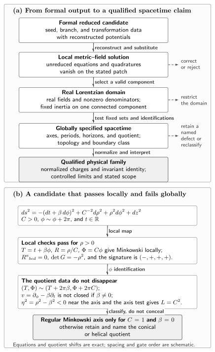
The upper panel separates increasingly strong claims: reconstruct the full fields, check the unreduced equations, select a connected real Lorentzian domain, supply axes, periods, horizons, quotients, topology, and boundary data, and only then interpret normalized charges, invariants, and controlled limits. The lower panel is exact. Its displayed metric is locally Minkowski with $\det G=-\rho^2$, yet the angular quotient gives a nonclosing degenerating direction or timelike angular circles when $\beta\ne0$ and elementary-flatness scalar $L=C^2$ when $\beta=0$. Only $C=1$ and $\beta=0$ has the standard regular Minkowski axis. Equations and quotient shifts are exact; the layout and order of checks are schematic.

Reconstruct before interpreting

A reduced potential is not yet a line element. For every transformation, retain enough information to reverse the reduction:

• the seed metric and matter fields, their coordinate and parameter domains, and the normalization and periods of all Killing generators;
• whether the reduction is timelike or spacelike, the base metric and orientation, and the definitions of twist and electromagnetic potentials;
• transformation parameters, branch choices, conjugation or reality conditions, pole data, integration constants, and reconstruction gauge; and
• the identity or inverse transformation expected to recover the seed.

These data distinguish a genuine discrepancy from a convention change. For example, reversing the base orientation reverses a reconstructed twist sign, while shifting a twist potential by a constant changes no metric. A rescaling of a projective soliton vector may cancel from the reconstructed fields entirely. None should be mistaken for new physics.

For four-dimensional stationary vacuum gravity, let $\xi=\partial_t$ be timelike on the reduction patch and set $f=-\xi^2>0$. A convenient decomposition is

$$ds^2=-f\,(dt+A)^2+f^{-1}h_{ij}\,dx^i dx^j, \qquad d\chi=f^2 *_h dA,$$

Here $h$ is the Riemannian metric on the three-dimensional orbit space and $*_h$ is its Hodge dual. The second equation fixes the twist convention, and the complex Ernst potential is $\mathcal E=f+i\chi$. A transformation of $\mathcal E$ gives $f$ and $\chi$, but the one-form $A$ must still be recovered by integrating the twist equation, and any remaining conformal or base equations must still be solved. This reconstruction step is explicit in Contopoulos et al. 2016, §§3–3.1, pp. 7–10, Eqs. (44)–(75), PDF.

Check the unreduced equations

After reconstruction, substitute the full fields into equations that did not participate in the generating identity. For the vacuum example,

$$R_{ab}=0.$$

For source-free Einstein–Maxwell theory with $\Lambda=0$, check

$$G_{ab}-8\pi G\,T^{\rm EM}_{ab}=0, \qquad \nabla_aF^{ab}=0, \qquad \nabla_{[a}F_{bc]}=0.$$

An exact symbolic check is strongest when every denominator and algebraic assumption is listed. Clearing a denominator is legitimate only on the region where it is nonzero; otherwise the operation can silently erase a boundary or exceptional branch. Numerical substitutions at generic admissible points are useful fault detectors, especially for very large expressions, but they do not prove an identity. Use them in addition to exact simplification, not instead of it.

Also check the equations integrated by quadrature. In inverse scattering, for example, the canonical determinant and matrix equation do not by themselves fix the conformal factor. In an Ehlers calculation, a correct transformed Ernst potential does not by itself prove that the reconstructed one-form has the intended sign and normalization.

Select a real Lorentzian component

State a connected set of inequalities, not merely a list of possible zeros:

• every radicand is real and every chosen root or pole branch is fixed;
• denominators introduced by the transformation and reconstruction are nonzero in the open region;
• coordinates have a declared ordering and range; and
• the real symmetric metric has exactly one negative eigenvalue.

The last condition is an inertia statement. On a connected region, a continuous nondegenerate metric cannot change its number of positive and negative eigenvalues. It is therefore enough to verify Lorentzian inertia at one point and prove $\det g\ne0$ throughout that component. The sign of $\det g$ alone is not enough: in four dimensions, both one and three negative eigenvalues give a negative determinant.

A zero of a displayed denominator is not automatically a curvature singularity. It may be an axis, a Killing horizon, a coordinate boundary, or the failure of a reduced chart where the reduction Killing field becomes null. Classify it by changing to a regular frame or chart and by checking curvature and matter fields. Never infer regularity merely because the reduced potentials remain finite.

Axes, horizons, and identifications

Let $v$ be a Killing generator whose norm $v^2$ tends to zero on a candidate axis. Define

$$L=\lim_{p\to\mathcal A} \frac{\nabla_a(v^2)\nabla^a(v^2)}{4v^2}.$$

If the orbit parameter of $v$ has period $\Delta\psi$, local polar geometry is smooth only when

$$\Delta\psi=\frac{2\pi}{\sqrt L}.$$

Thus $L=1$ is the elementary-flatness test only after a $2\pi$ period has been fixed. It is a necessary local condition, not a complete global one: the integral curves of $v$ must close with that period, disconnected axis segments must obey one compatible set of identifications, and any corner of a higher-dimensional axial torus must satisfy the appropriate primitive-lattice condition. Ergoregions, Killing Horizons, and Axis Structure develops these local tests; Inverse Scattering and Soliton Metrics applies their higher-dimensional rod version.

A candidate horizon needs more than $g^{rr}=0$. Verify that the proposed hypersurface is null, identify a constant Killing generator when one exists, exhibit a horizon-penetrating chart or regular frame, and check that the metric and matter invariants remain finite there. This page needs only enough horizon information to classify the exact family; horizon mechanics belongs to Black-Hole Geometry and Mechanics.

From local charts to topology

A local line element does not determine the global manifold. Begin with the connected components left after genuine singular sets and excluded denominators are removed. Then record the chart overlaps and transition maps, the fixed-point sets of the symmetry action, the quotient group and its period lattice, the end structure, and any cycles that cannot be contracted. Axis and horizon cross-sections should be identified from these data rather than guessed from coordinate names.

The Taub–NUT example below makes the procedure concrete. Its north and south charts are locally regular, but their transition map shifts time when $\phi$ winds once. Choosing whether that shift is an identification changes both chronology and the topology of the constant-$r$ hypersurfaces. The topology is therefore part of the completion data, not an output of $R_{ab}=0$.

Normalize the boundary class before reading charges

Solution-generating maps often change the asymptotic frame or even the asymptotic class. Before reading coefficients as charges:

1. remove only constant time–angle mixing and coordinate scalings that preserve the declared quotient lattice and the normalization of the asymptotic generators;
2. fix angular periods and the normalization of the asymptotic time translation;
3. fix electromagnetic and twist gauges;
4. state the actual boundary class; and
5. use the surface integral or asymptotic expansion appropriate to that class.

An external Melvin field, acceleration defect, Kaluza–Klein circle, or NUT fibration is not failed asymptotic flatness when it is intentionally retained. It is a different boundary condition. Conversely, a parameter appearing beside $dt\,d\phi$ is not automatically angular momentum; it may be removable by a frame change or forced by a quotient.

Parameter counting comes last. Compute the rank of the map from seed and transformation data to normalized charges and invariants, then quotient explicit coordinate, gauge, discrete, pole-permutation, and projective-vector redundancies. A zero-parameter limit should recover the seed as a metric with the same declared identifications. If a finite limit requires a simultaneous coordinate rescaling, record the held-fixed combinations rather than performing a naive substitution.

Curvature tests are necessary but not complete

Curvature blow-up is strong evidence for a genuine singularity, but finite scalar polynomial invariants do not prove regularity. Nor do equal finite invariants prove local equivalence in every spacetime class. Degenerate Kundt geometries are the standard exceptional sector to the generic invariant-characterization result Coley, Hervik, and Pelavas 2009, §§1–3 and §§7–9, pp. 1–7 and 21–36, PDF.

A compact control example is the Ricci-flat plane wave

$$ds^2=-2\,du\,dv+dx^2+dy^2 +A(u)(x^2-y^2)\,du^2.$$

When $A(u)\ne0$, components such as $R_{uxux}=-A(u)$ are nonzero, so the spacetime is not flat; nevertheless its polynomial curvature scalars vanish. Scalar invariants therefore belong in a larger set of checks that can include a regular frame, parallelly propagated curvature, Cartan–Karlhede data—canonical frame components and their derivatives—geodesic behavior, and quotient structure.

Worked verification: Schwarzschild to Taub–NUT

The Ehlers transformation gives a compact example in which every layer matters. It passes reconstruction, Ricci-flatness, Lorentzian-signature, and local horizon checks. Yet its north and south axis patches and nondecaying $g_{t\phi}$ prevent the result from being interpreted as an ordinary asymptotically flat black-hole exterior; the target is the distinct Taub–NUT spacetime.

Let the Schwarzschild seed use a mass length $m>0$ and radius $x>2m$:

$$\mathcal E_0=f_0=1-\frac{2m}{x}.$$

Choose the normalized real-parameter representative

$$\mathcal E_\lambda =\frac{\mathcal E_0+i\lambda}{1+i\lambda\mathcal E_0}, \qquad \mathcal E_\lambda\longrightarrow1 \quad(x\to\infty).$$

The normalization at infinity is important: an unnormalized fractional-linear map can change the scale of the asymptotic time coordinate. Its real and imaginary parts are

$$f_\lambda =\frac{(1+\lambda^2)f_0}{1+\lambda^2f_0^2}, \qquad \chi_\lambda =\frac{\lambda(1-f_0^2)}{1+\lambda^2f_0^2}.$$

Define

$$M=m\,\frac{1-\lambda^2}{1+\lambda^2}, \qquad n=\frac{2m\lambda}{1+\lambda^2}, \qquad r=x-\frac{2m\lambda^2}{1+\lambda^2},$$

and

$$\Sigma=r^2+n^2, \qquad \Delta=r^2-2Mr-n^2.$$

Here $M$ is the transformed mass coefficient in this normalization and $n$ is the NUT parameter; both have dimensions of length. For the positive-$M$ branch one may take $|\lambda|<1$. Direct algebra gives

$$M^2+n^2=m^2, \qquad f_\lambda=\frac{\Delta}{\Sigma}, \qquad \chi_\lambda=\frac{2n(r-M)}{\Sigma}.$$

The three-dimensional base inherited from Schwarzschild becomes

$$h=dr^2+\Delta\,(d\theta^2+\sin^2\theta\,d\phi^2).$$

With orientation $dr\wedge d\theta\wedge d\phi$, the one-form

$$A=2n\cos\theta\,d\phi$$

satisfies $d\chi=f^2 *_h dA$. Reconstruction therefore gives

$$ds^2 =-\frac{\Delta}{\Sigma} \bigl(dt+2n\cos\theta\,d\phi\bigr)^2 +\frac{\Sigma}{\Delta}\,dr^2 +\Sigma\,(d\theta^2+\sin^2\theta\,d\phi^2).$$

This is the Lorentzian Taub–NUT family in the site convention. The construction and its monopole-like interpretation are discussed in Bičák 2000, §7, printed pp. 62–66, PDF; coordinate, axis, and extension details are treated in Griffiths and Podolský 2009, §12.1, printed pp. 214–228.

Local equation and domain checks

Direct substitution gives the representative identities

$$\det g=-\Sigma^2\sin^2\theta, \qquad \frac{d\chi}{dr} =-\frac{2n\Delta}{\Sigma^2} =f^2(*_h dA)_r.$$

The downloadable exact SymPy checker constructs the Christoffel symbols and full Riemann tensor from the displayed metric, simplifies all ten independent Ricci components to zero, and verifies the orientation-sensitive Hodge dual. It requires Python 3 and SymPy; no numerical sampling is used for those identities. On the connected exterior component

$$r>r_+=M+\sqrt{M^2+n^2}=M+m,$$

$\Delta>0$ and $\Sigma>0$, so the displayed chart has one negative and three positive directions. The seed boundary $x=2m$ maps exactly to $r=r_+$.

The apparent divergence of $g_{rr}$ at $\Delta=0$ is removable locally. Defining

$$dv=dt+\frac{\Sigma}{\Delta}\,dr$$

gives

$$ds^2 =-\frac{\Delta}{\Sigma} \bigl(dv+2n\cos\theta\,d\phi\bigr)^2 +2\,dr\bigl(dv+2n\cos\theta\,d\phi\bigr) +\Sigma\,d\Omega_2^2,$$

which is finite at $r=r_+$. This establishes local horizon regularity in a suitable angular patch. It does not settle the global axis patching.

The remaining horizon tests are explicit:

$$g^{-1}(dr,\,dr)=\frac{\Delta}{\Sigma}, \qquad g(\partial_v,\partial_v)=-\frac{\Delta}{\Sigma}, \qquad \det g_{(v,r,\theta,\phi)}=-\Sigma^2\sin^2\theta.$$

Thus $r=r_+$ is null, $\partial_v=\partial_t$ is its null Killing generator in this patch, and the ingoing metric remains nondegenerate away from the polar-coordinate axes. This is a local extension statement, not a claim about a preferred global Taub–NUT completion.

The global axis test changes the conclusion

At the north and south axes, the kernels of the $(t,\phi)$ Killing block are

$$v_N=\partial_\phi-2n\,\partial_t, \qquad v_S=\partial_\phi+2n\,\partial_t.$$

Each satisfies the local elementary-flatness limit with a $2\pi$ angular parameter. But if $t$ is nonperiodic, neither helical generator has a closed orbit in the original coordinates. Equivalently, regular north and south times may be chosen as

$$t_N=t+2n\phi, \qquad t_S=t-2n\phi.$$

On their overlap, $t_N-t_S=4n\phi$. Since $\phi\sim\phi+2\pi$, removing both axial strings by this two-patch construction requires a time period

$$\Delta t=8\pi |n|.$$

Then the stationary time orbits are closed and timelike wherever $\Delta>0$, because $g_{tt}=-\Delta/\Sigma<0$. The same choice changes topology: $t/(2n)$ has the $4\pi$ period of an Euler angle, so each fixed-$r$ hypersurface is the $S^3$ Hopf fibration rather than $S^2\times\mathbb R$. With nonperiodic time, the bundle and retained-string prescription are different.

The transformation has produced a correct local vacuum solution, but not an ordinary asymptotically flat black-hole exterior. One must state which global prescription is intended: periodic time with its closed timelike curves, a retained axial string, or a carefully specified nonperiodic-time treatment. Bičák gives the standard periodic-patch conclusion in Bičák 2000, §7.2, printed pp. 64–66, PDF; a distinct transparent-string prescription and its claimed scope are developed in Clément, Gal’tsov, and Guenouche 2015, §§I and IV–V, pp. 1–2 and 5–8, PDF.

Charges, invariants, and the identity limit

The large-$r$ coefficients are

$$\lim_{r\to\infty}\frac r2(1+g_{tt})=M, \qquad \lim_{r\to\infty}\frac r2\,\chi=n, \qquad g_{t\phi}\longrightarrow-2n\cos\theta.$$

The nondecaying last term is the warning: $n$ changes the asymptotic fibration, so $M$ should not be called an ordinary asymptotically flat ADM mass without qualification.

The parameter map is locally invertible on the chosen finite-$\lambda$ branch:

$$\det\frac{\partial(M,n)}{\partial(m,\lambda)} =\frac{2m}{1+\lambda^2}, \qquad m=\sqrt{M^2+n^2}, \qquad \lambda=\frac{n}{m+M}.$$

Thus $\lambda$ is a locally independent continuous parameter once the axial orientation and time orientation are fixed; it rotates the seed mass into mass and NUT coefficients along $M^2+n^2=m^2$. There is still a discrete qualification: $\lambda\mapsto-\lambda$ sends $n\mapsto-n$, and an axial parity reversal $\phi\mapsto-\phi$ maps the resulting unoriented metric back to the original one. If axial orientation is not part of the data, the final parameter space should quotient this sign relation rather than count it twice.

One useful curvature magnitude is

$$\sqrt{K^2+P^2} =\frac{48(M^2+n^2)}{(r^2+n^2)^3},$$

where $K=R_{abcd}R^{abcd}$ and $P={}^*R_{abcd}R^{abcd}$ in the vacuum region. The downloadable checker contracts both invariants and verifies this combination exactly. It is finite at $r=0$ when $n\ne0$, but that fact does not remove the quotient and chronology problems just found. Finally,

$$\lambda\to0: \qquad n\to0,\quad M\to m,\quad r\to x,$$

the local metric and coordinate range return directly to Schwarzschild without a singular coordinate change. The global statement depends on the prescription. With nonperiodic time and a retained or transparent string, the declared time and angular identifications also return to the Schwarzschild ones. In the periodic Misner completion, however, $\Delta t=8\pi|n|\to0$; that quotient does not approach ordinary Schwarzschild with a noncompact time. The local identity limit passes, while the global limit must be reported separately.

Exact counterexample: locally flat is not globally regular

Now consider the lower panel of the figure:

$$ds^2=-(dt+\beta\,d\phi)^2 +C^{-2}d\rho^2+\rho^2d\phi^2+dz^2, \qquad C>0,\quad \phi\sim\phi+2\pi,\quad t\in\mathbb R.$$

For $\rho>0$, the change

$$T=t+\beta\phi, \qquad R=\frac{\rho}{C}, \qquad \Phi=C\phi, \qquad Z=z$$

puts the metric in Minkowski form. Hence $R^a{}_{bcd}=0$ on the punctured region, and the stationary Killing block satisfies the canonical-looking condition $\det G=-\rho^2$. Neither fact decides the quotient.

Under one angular turn,

$$(T,\Phi)\sim(T+2\pi\beta,\Phi+2\pi C).$$

The locally degenerating vector is

$$v=\partial_\phi-\beta\partial_t, \qquad v^2=\rho^2.$$

If $\beta\ne0$ and $t$ is nonperiodic, its integral curves do not close. The actually closed angular generator $\eta=\partial_\phi$ instead has

$$\eta^2=\rho^2-\beta^2,$$

so its circles are timelike for $0<\rho<|\beta|$. If $\beta=0$, the closed generator does degenerate, and its elementary-flatness scalar is

$$\lim_{\rho\to0} \frac{\nabla_a(\eta^2)\nabla^a(\eta^2)}{4\eta^2} =C^2.$$

For $\beta=0$, $C$ is the circumference-to-radius conicity relative to a regular plane. With the fixed $2\pi$ period, the axis is regular only for $C=1$: $C<1$ gives a deficit and $C>1$ an excess. This example, adapted from Griffiths and Podolský 2009, §§3.4–3.4.1, printed pp. 35–37, proves the central lesson with an exact flat local metric: field equations, curvature scalars, signature, and a canonical determinant can all pass while the global spacetime fails the stated regular-axis or chronology requirement.

A reusable verification sequence

For a new generated candidate, report the result in this order:

1. Generation data: seed, equations, symmetries, reduction signs, orientation, transformation branches, gauges, and identity map.
2. Reconstruction: full metric and matter fields, remaining quadratures, and excluded denominators.
3. Unreduced equations: exact residuals, assumptions used in simplification, and any secondary numerical spot checks.
4. Domain: connected coordinate and parameter inequalities, reality, inertia, and boundary classification.
5. Global data: charts, axes, periods, horizon generators and regular charts, quotient identifications, topology, and boundary class.
6. Interpretation: normalized charges, independent invariants or Cartan data, parameter-map rank, redundancies, singularities, and controlled limits.
7. Claim boundary: what has not been established—typically maximality, uniqueness, stability, formation, or observational relevance.

This ordering prevents a common reversal: naming a parameter first and looking for evidence of its meaning afterward.

Common pitfalls

“Ricci-flat” means “acceptable.” Ricci-flatness is a local differential statement. Axial closure, conical regularity, chronology, topology, and boundary conditions are additional data.

A negative determinant proves Lorentzian signature. It does not in four dimensions: one and three negative eigenvalues both give $\det g<0$. Establish the inertia on a connected nondegenerate component.

Finite curvature scalars prove smoothness. Scalar invariants can miss quotient defects, incomplete or parallelly propagated behavior, and nonflat degenerate-Kundt fields. Use the diagnostic appropriate to the suspected failure.

Every displayed parameter is physical. A parameter becomes physical only after coordinate and gauge redundancies, periods, asymptotic normalization, and the rank of the map to invariant data have been resolved.

Exercises

1. The Ehlers charge circle

Starting from

$$M=m\frac{1-\lambda^2}{1+\lambda^2}, \qquad n=\frac{2m\lambda}{1+\lambda^2},$$

prove $M^2+n^2=m^2$, compute the Jacobian of $(m,\lambda)\mapsto(M,n)$, and invert the map on $m>0$, $|\lambda|<1$.

Solution

Squaring and adding gives

$$M^2+n^2 =m^2\frac{(1-\lambda^2)^2+4\lambda^2}{(1+\lambda^2)^2} =m^2.$$

Direct differentiation yields

$$\det\frac{\partial(M,n)}{\partial(m,\lambda)} =\frac{2m}{1+\lambda^2}>0.$$

Thus the parameters are locally independent on the stated branch. Since $m>0$,

$$m=\sqrt{M^2+n^2}.$$

Moreover,

$$m+M=\frac{2m}{1+\lambda^2},$$

so

$$\lambda=\frac{n}{m+M}.$$

The denominator is positive for $|\lambda|<1$. Thus $\lambda$ is locally recoverable and continuously nonredundant when the time and axial orientations are fixed. If axial parity is identified, however, $\lambda$ and $-\lambda$ describe the same unoriented metric after $\phi\mapsto-\phi$; the discrete sign must then be quotiented rather than counted twice.

2. One determinant, opposite inertias

Give two real diagonal Lorentzian four-metrics with the same negative determinant but opposite inertia. Explain how the site’s signature convention, a seed metric, and connectedness repair this ambiguity.

Solution

For example,

$$g_1=\operatorname{diag}(-1,1,1,1), \qquad g_2=\operatorname{diag}(-1,-1,-1,1)$$

both have determinant $-1$. The first has inertia $(1,3)$—one negative and three positive directions—while the second has inertia $(3,1)$. Both are Lorentzian, but they use opposite sign conventions; the site’s $(-,+,+,+)$ convention selects $g_1$. The determinant sign alone does not make that selection.

If a continuous family begins at a known Lorentzian seed and remains real, symmetric, and nondegenerate on a connected parameter–coordinate component, none of its eigenvalues can cross zero. Its inertia is constant there. Checking the inertia at one point plus $\det g\ne0$ throughout that connected component is then sufficient.

3. Period and chronology in the spinning quotient

For

$$ds^2=-(dt+\beta\,d\phi)^2+C^{-2}d\rho^2+\rho^2d\phi^2+dz^2,$$

show that the degenerating vector $v=\partial_\phi-\beta\partial_t$ has elementary-flatness scalar $L=C^2$. What period would make its local polar plane smooth? Why does that not solve the $\beta\ne0$ quotient with nonperiodic $t$?

Solution

The norm is $v^2=\rho^2$. Since $g^{\rho\rho}=C^2$,

$$L=\lim_{\rho\to0} \frac{\nabla_a(v^2)\nabla^a(v^2)}{4v^2} =\lim_{\rho\to0}\frac{C^2(2\rho)^2}{4\rho^2} =C^2.$$

The local smoothness period is therefore

$$\Delta\psi=\frac{2\pi}{C}.$$

But an integral curve of $v$ changes $(t,\phi)$ by $(-\beta\Delta\psi,\Delta\psi)$. With nonperiodic $t$, it does not close when $\beta\ne0$. Imposing an additional helical identification changes the global spacetime and introduces a periodic time component. Meanwhile the original closed $\phi$ circles have norm $\rho^2-\beta^2$ and are timelike near the axis. The local elementary-flatness ratio cannot cure the global quotient.

4. A nonflat metric with a vanishing quadratic invariant

For

$$ds^2=-2\,du\,dv+dx^2+dy^2 +A(u)(x^2-y^2)\,du^2,$$

verify that the vacuum equation holds, identify a nonzero curvature component, and explain why $R_{abcd}R^{abcd}=0$.

Solution

Write $H=A(u)(x^2-y^2)$. A Brinkmann wave obeys

$$R_{uu}=-\frac12(H_{,xx}+H_{,yy}).$$

Here $H_{,xx}=2A$ and $H_{,yy}=-2A$, so $R_{uu}=0$ and all other Ricci components vanish. Nevertheless,

$$R_{uxux}=-\frac12H_{,xx}=-A(u), \qquad R_{uyuy}=-\frac12H_{,yy}=A(u),$$

so the metric is nonflat whenever $A(u)\ne0$.

Every nonzero Riemann component has two lower $u$ indices. Raising a $u$ index uses $g^{uv}$ because $g^{uu}=0$, but there are no corresponding curvature components with a lower $v$ index. Every complete quadratic contraction therefore vanishes. The Kretschmann scalar cannot distinguish this wave from Minkowski space.

References

• Bičák, Jiří. “Selected Solutions of Einstein’s Field Equations: Their Role in General Relativity and Astrophysics.” In Einstein’s Field Equations and Their Physical Implications, edited by Bernd G. Schmidt, Lecture Notes in Physics 540, 1–126. Berlin: Springer, 2000. DOI; arXiv:gr-qc/0004016.
• Clément, Gérard, Dmitri Gal’tsov, and Mourad Guenouche. “Rehabilitating Space-Times with NUTs.” Physics Letters B 750 (2015): 591–594. DOI; Open PDF.
• Coley, Alan, Sigbjørn Hervik, and Nicos Pelavas. “Spacetimes Characterized by Their Scalar Curvature Invariants.” Classical and Quantum Gravity 26 (2009): 025013. DOI; Open PDF.
• Contopoulos, I. G., F. P. Esposito, K. Kleidis, D. B. Papadopoulos, and L. Witten. “Generating Solutions to the Einstein Field Equations.” International Journal of Modern Physics D 25, no. 2 (2016): 1650022. DOI; Open PDF.
• Griffiths, Jerry B., and Jiří Podolský. Exact Space-Times in Einstein’s General Relativity. Cambridge: Cambridge University Press, 2009. DOI.