Inverse Scattering and Soliton Metrics

Inverse scattering turns the nonlinear stationary vacuum equations into the compatibility condition of a linear system. A pole in the auxiliary spectral plane does not by itself equal a mass or an angular momentum: its axis position fixes geometric transition data, while its constant polarization vector changes how the Killing directions are mixed. Only after reconstructing the metric, restoring $\det G=-\rho^2$, choosing an asymptotic frame, and passing global regularity tests do combinations of the pole data become physical parameters.

This page develops that algebra and then carries it through a complete benchmark: a determinant-preserving two-pole transformation of the five-dimensional Tangherlini solution into the doubly spinning Myers–Perry black hole.

Required background. Killing Fields and Isometry Groups supplies the commuting Killing generators and their Gram matrix.

Helpful background. Einstein’s Equation supplies the vacuum equations; The Riemann Curvature Tensor supplies invariant regularity checks; Exact Solutions of Einstein’s Equations supplies benchmark families; Formulations of General Relativity supplies two-dimensional reduction; and PDEs and Green Functions supplies compatibility systems and boundary data.

Scope. The Belinski–Zakharov construction below assumes $D$-dimensional Ricci-flat gravity with $\Lambda=0$, $D-2$ commuting Killing fields, and an orthogonally transitive action—that is, two-surfaces orthogonal to the Killing orbits exist—on the patch considered. The standard stationary-axisymmetric $D=4$ and biaxisymmetric $D=5$ black-hole families meet this condition. In $D=5$, the second axial $U(1)$ is an additional symmetry hypothesis rather than a consequence of stationarity alone. For $D\ge6$, the condition selects still more special sectors—often with additional compact directions—and excludes a generic Myers–Perry black hole. The worked example is the nonextremal five-dimensional black-hole branch. Weyl–Papapetrou Form and Orbit Space supplies the four-dimensional specialization; Ergoregions, Killing Horizons, and Axis Structure develops the interval interpretation used after dressing.

The reduced vacuum equation

Choose coordinates $x^A$ along the $D-2$ Killing fields and canonical coordinates $(\rho,z)$ on the two-dimensional orbit space:

$$ds^2=G_{AB}(\rho,z)\,dx^A dx^B +e^{2\nu(\rho,z)}(d\rho^2+dz^2), \qquad \det G=-\rho^2.$$

The symmetric matrix $G$ is the Gram matrix of the Killing fields. In a stationary region it has one negative eigenvalue. Define

$$U=\rho(\partial_\rho G)G^{-1}, \qquad V=\rho(\partial_zG)G^{-1}.$$

Then the vacuum equations split into the matrix equation

$$\partial_\rho U+\partial_zV=0$$

and two first-order equations for the conformal factor:

$$\begin{aligned} \partial_\rho\log e^{2\nu} &=-\frac1\rho+\frac{1}{4\rho} \operatorname{Tr}(U^2-V^2),\\ \partial_z\log e^{2\nu} &=\frac{1}{2\rho}\operatorname{Tr}(UV). \end{aligned}$$

The matrix equation makes these quadratures compatible, but it does not fix the multiplicative constant in $e^{2\nu}$. Axis regularity or asymptotic normalization fixes that constant. This reduction, including the higher-dimensional determinant condition, is derived in Emparan and Reall 2008, §5.2, pp. 28–29, Eqs. (66)–(70), PDF.

The Lax pair

Introduce a $(D-2)\times(D-2)$ matrix $\Psi(\lambda,\rho,z)$ normalized by

$$\Psi(0,\rho,z)=G(\rho,z).$$

It obeys

$$\mathcal D_z\Psi= \frac{\rho V-\lambda U}{\lambda^2+\rho^2}\Psi, \qquad \mathcal D_\rho\Psi= \frac{\rho U+\lambda V}{\lambda^2+\rho^2}\Psi,$$

where

$$\mathcal D_z=\partial_z- \frac{2\lambda^2}{\lambda^2+\rho^2}\partial_\lambda, \qquad \mathcal D_\rho=\partial_\rho+ \frac{2\lambda\rho}{\lambda^2+\rho^2}\partial_\lambda.$$

Before these operators act, $\lambda$ is independent of $\rho$ and $z$. The $\partial_\lambda$ terms make the characteristic value of $\lambda$ move over the orbit space. Define the two matrix coefficients

$$\mathcal A_z=\frac{\rho V-\lambda U}{\lambda^2+\rho^2}, \qquad \mathcal A_\rho=\frac{\rho U+\lambda V}{\lambda^2+\rho^2},$$

Then the zero-curvature condition

$$[\mathcal D_z-\mathcal A_z,\mathcal D_\rho-\mathcal A_\rho]\Psi=0$$

is equivalent to the reduced vacuum equation. The nonlinear problem has therefore become the compatibility condition of a linear system. Belinski and Zakharov give the original construction in Belinski and Zakharov 1978, §§2–4, pp. 986–990, official PDF; their stationary-axisymmetric continuation is Belinski and Zakharov 1979, §§1–3, pp. 1–5, official PDF.

From pole data to a metric

Let $G_0$ be a seed and $\Psi_0$ its solution of the Lax pair. A rational $n$-pole dressing has

$$\Psi=\chi\Psi_0, \qquad \chi(\lambda)=I+ \sum_{k=1}^n\frac{R_k}{\lambda-\widetilde\mu_k}.$$

For a real axis point $a_k$, define

$$\begin{aligned} \mu_k&=\sqrt{\rho^2+(z-a_k)^2}-(z-a_k),\\ \bar\mu_k&=-\sqrt{\rho^2+(z-a_k)^2}-(z-a_k) =-\frac{\rho^2}{\mu_k}. \end{aligned}$$

A pole trajectory $\widetilde\mu_k$ is chosen to be either $\mu_k$ (a soliton) or $\bar\mu_k$ (an antisoliton). On the axis, $\mu_k$ vanishes to the right of $a_k$, whereas $\bar\mu_k$ vanishes to its left. Thus the branch choice is geometric data, not a sign that can be changed silently.

The residues need not be found by integrating another differential equation. Choose constant row vectors $m_0^{(k)}$ and form

$$m^{(k)a} =m_{0b}^{(k)} \left[\Psi_0^{-1}(\widetilde\mu_k,\rho,z)\right]^{ba}.$$

Next define

$$N_a^{(k)}=(G_0)_{ab}m^{(k)b}, \qquad \Gamma_{kl}= \frac{m^{(k)a}(G_0)_{ab}m^{(l)b}} {\rho^2+\widetilde\mu_k\widetilde\mu_l}.$$

If $\Gamma$ is invertible, the dressed Killing block is

$$G_{ab} =(G_0)_{ab} -\sum_{k,l=1}^n \frac{(\Gamma^{-1})_{kl}} {\widetilde\mu_k\widetilde\mu_l} N_a^{(k)}N_b^{(l)}.$$

These equations are the missing bridge between “add a pole” and “obtain a metric.” Pole positions enter through $\widetilde\mu_k$; polarizations enter through $m_0^{(k)}$; and every off-diagonal metric component is produced by the finite matrix inverse $\Gamma^{-1}$. The stationary reconstruction formulas appear in Belinski and Zakharov 1979, §2 and Appendix, pp. 2–8, official PDF and in dimension-independent form in Pomeransky 2006, §II, pp. 3–6, Eqs. (1)–(12), PDF.

For a real symmetric seed, a seed wavefunction chosen real along the real pole trajectories, and real polarization vectors, $\Gamma$ is real symmetric and the displayed reconstruction makes $G$ real symmetric as well. If complex data are used, the pole and polarization set must instead be closed under the Belinski–Zakharov conjugation and involution conditions; otherwise the algebraic output need not be a real metric.

Rescaling one polarization by any nonzero constant, $m_0^{(k)}\mapsto c_km_0^{(k)}$ with $c_k\ne0$, changes the corresponding row and column of $\Gamma$ but cancels out of $G$. Raw vector components are therefore homogeneous coordinates, not yet physical charges.

It helps to keep the different pieces of “pole data” separate:

Datum	Algebraic role	Redundancy or physical interpretation
$a_k$	Constant location of a branch point on the $z$-axis	A common translation of all $a_k$ can be absorbed into $z$; separations can become invariant interval lengths after global normalization.
$\mu_k$ or $\bar\mu_k$	Coordinate-dependent characteristic trajectory	The branch fixes which half-axis carries its zero and cannot be changed without changing the construction.
$[m_0^{(k)}]$	Projective orientation mixed into the Killing block	Overall scale is redundant; surviving ratios can become rotation or NUT parameters only after the asymptotic frame is fixed.
$R_k$	Rank-one residue of the dressing matrix	Computed from the seed, pole, and polarization; it is not additional free data.
Constant in $e^{2\nu}$	Normalization of the orbit-space metric	Fixed by asymptotic or axis regularity, not by the Lax compatibility condition.

Why poles must be removed and re-added

A direct $n$-pole dressing changes the determinant by

$$\det G =(-1)^n\rho^{2n} \left(\prod_{k=1}^n\widetilde\mu_k^{-2}\right) \det G_0.$$

In four dimensions one can often repair this with a scalar rescaling of the $2\times2$ block. In $D>4$, multiplying all of $G$ by a fractional determinant power generally creates fractional rod densities and curvature singularities. The determinant condition is not cosmetic.

The reliable higher-dimensional procedure is:

1. start with a physical seed;
2. remove chosen poles using trivial basis-aligned polarizations;
3. solve for the diagonal intermediate wavefunction;
4. re-add the same pole branches at the same positions with tilted polarizations; and
5. restore the physical scale and asymptotic Killing frame.

The removal and re-addition have identical determinant factors, so they cancel. For the same pole set, the conformal factor can be recovered without a fresh integration:

$$e^{2\nu} =e^{2\nu_{\rm seed}} \frac{\det\Gamma}{\det\Gamma_{\rm triv}},$$

with the remaining constant fixed at infinity. Emparan and Reall explain the determinant obstruction and this remove–re-add method in Emparan and Reall 2008, §5.2.2, pp. 32–33, Eqs. (97)–(100), PDF.

The figure shows the two distinct roles of the data. Inspect the unchanged endpoints and axis rods, then compare the static and rotating horizon directions.

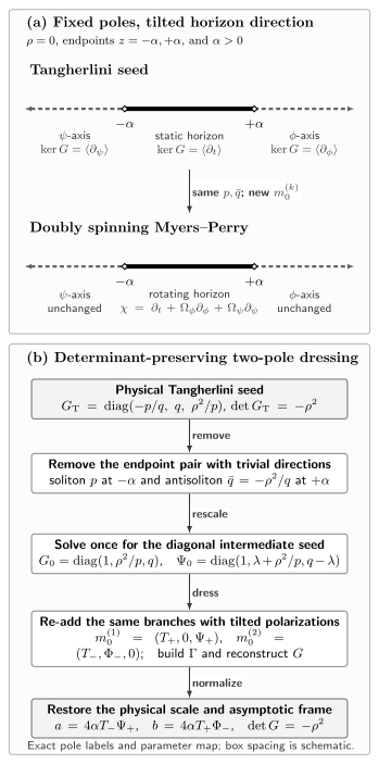
Determinant-preserving two-pole dressing for the nonextremal five-dimensional benchmark. Here $p$ is the soliton branch at $z=-\alpha$, $q$ is the soliton branch at $z=+\alpha$, and $\bar q=-\rho^2/q$ is the antisoliton branch re-added at the right endpoint. The two pole locations remain fixed at the endpoints and hence preserve the three-interval decomposition, while $m_0^{(1)}=(T_+,0,\Psi_+)$ and $m_0^{(2)}=(T_-,\Phi_-,0)$ mix time with the two axial directions. After determinant and frame normalization, the finite rod tilts from $\partial_t$ to $\chi=\partial_t+\Omega_\phi\partial_\phi+\Omega_\psi\partial_\psi$, with $a=4\alpha T_-\Psi_+$ and $b=4\alpha T_+\Phi_-$. Interval positions, branch labels, and parameter maps are exact; vertical spacing and box layout are schematic, not proper distance or a causal diagram.

Worked benchmark: Tangherlini to Myers–Perry

The example follows Pomeransky 2006, §III, pp. 6–9, Eqs. (13)–(23), PDF. Pomeransky writes the reduced right-hand side as $-ds_{\rm P}^2$; identifying it with our mostly-plus line element translates the source’s overall signature exactly once. Direct substitution of the source’s Eqs. (9)–(17) reveals a sign inconsistency between its printed Eq. (20) and the negative rotational cross terms displayed immediately afterward in Eq. (21). The frame used below is the printed Eq. (20) followed by reversal of both final axial coordinates; it is the choice that makes the direct BZ reconstruction agree with Eq. (21) and the standard mostly-plus orientation of Myers–Perry. The reversals preserve the $2\pi$ periods.

Work in $D=5$ with Killing basis $(\partial_t,\partial_\phi,\partial_\psi)$ and $2\pi$ periods for the final axial coordinates. In five-dimensional canonical coordinates, $\rho$, $z$, and the endpoint parameter $\alpha$ have dimensions of length squared.

1. Fix the seed and both branches

Put the two endpoints at $z=-\alpha$ and $z=+\alpha$, with $\alpha>0$, and abbreviate

$$\begin{aligned} p&=\sqrt{\rho^2+(z+\alpha)^2}-(z+\alpha),\\ q&=\sqrt{\rho^2+(z-\alpha)^2}-(z-\alpha),\\ \bar q&=-\frac{\rho^2}{q}. \end{aligned}$$

The five-dimensional Tangherlini Killing block and base factor are

$$G_{\rm T} =\operatorname{diag}\left(-\frac pq,\ q,\ \frac{\rho^2}{p}\right),$$ $$e^{2\nu_{\rm T}} =\frac{q(\rho^2+pq)} {(\rho^2+p^2)(\rho^2+q^2)}.$$

Its finite interval $-\alpha<z<\alpha$ is a static horizon rod; the two semi-infinite intervals are the $\psi$- and $\phi$-axes.

Remove the soliton $p$ with the trivial $\psi$-direction $(0,0,1)$ and the antisoliton $\bar q$ with the trivial $\phi$-direction $(0,1,0)$, then make the convenient intermediate rescaling used by Pomeransky. The resulting diagonal, nonphysical seed and its wavefunction are

$$G_0=\operatorname{diag}\left(1,\frac{\rho^2}{p},q\right), \qquad \Psi_0(\lambda)= \operatorname{diag}\left( 1,\lambda+\frac{\rho^2}{p},q-\lambda \right).$$

Now re-add the same branches

$$\widetilde\mu_1=p, \qquad \widetilde\mu_2=\bar q,$$

but use

$$m_0^{(1)}=(T_+,0,\Psi_+), \qquad m_0^{(2)}=(T_-,\Phi_-,0).$$

Evaluation of $\Psi_0^{-1}$ at the two poles gives

$$\begin{aligned} m^{(1)} &=\left(T_+,0,\frac{\Psi_+}{q-p}\right),\\ m^{(2)} &=\left( T_-, \frac{\Phi_-pq}{\rho^2(q-p)}, 0 \right). \end{aligned}$$

At this point $\Gamma$, $G$, and $e^{2\nu}$ follow from finite-dimensional algebra. The next expandable calculation makes that bridge explicit without interrupting the main geometric argument.

The finite Gram-matrix calculation

Write $\delta=q-p$. Multiplication by the diagonal seed gives

$$N^{(1)}=\left(T_+,0,\frac{q\Psi_+}{\delta}\right), \qquad N^{(2)}=\left(T_-,\frac{q\Phi_-}{\delta},0\right).$$

The three independent entries of the symmetric $2\times2$ Gram matrix are

$$\begin{aligned} \Gamma_{11} &=\frac{T_+^2+q\Psi_+^2/\delta^2}{\rho^2+p^2},\\ \Gamma_{12}=\Gamma_{21} &=\frac{qT_+T_-}{\rho^2\delta},\\ \Gamma_{22} &=\frac{T_-^2+p q^2\Phi_-^2/(\rho^2\delta^2)} {\rho^2+\rho^4/q^2}. \end{aligned}$$

Substituting this $\Gamma^{-1}$ and the two $N$ vectors into the reconstruction formula produces the complete intermediate Killing block. No differential equation remains at this stage.

Multiplying the reconstructed intermediate block by $-p/q$ restores the physical scale; setting $T_+=T_-=0$ restores $G_{\rm T}$ exactly.

2. Identify the physical parameters and frame

On the regular black-hole branch, where the expression below is positive, choose nonzero real projective rescalings of $m_0^{(1)}$ and $m_0^{(2)}$ so that

$$\Psi_+^2\Phi_-^2 -16\alpha^2T_+^2T_-^2=1.$$

The product of the two rescalings fixes this normalization; their relative rescaling remains redundant and does not change the reconstructed metric.

The combinations that survive in the asymptotically normalized metric are

$$\begin{aligned} \mu &=4\alpha \left(4\alpha T_+^2+\Psi_+^2\right) \left(4\alpha T_-^2+\Phi_-^2\right),\\ a&=4\alpha T_-\Psi_+, \qquad b=4\alpha T_+\Phi_-. \end{aligned}$$

They obey

$$16\alpha^2 =(\mu-a^2-b^2)^2-4a^2b^2.$$

Thus the polarization data have become the two rotation lengths $a$ and $b$, while the endpoint half-length $\alpha$ is fixed by the Myers–Perry discriminant.

The last step is a constant change from the BZ Killing basis to the asymptotic frame:

$$\begin{aligned} t_{\rm BZ}&=t-a\phi-b\psi,\\ \phi_{\rm BZ} &=-\Psi_+\Phi_-\,\phi +4\alpha T_+T_-\,\psi,\\ \psi_{\rm BZ} &=-\Psi_+\Phi_-\,\psi +4\alpha T_+T_-\,\phi. \end{aligned}$$

This is Pomeransky’s printed Eq. (20) followed by $\phi\mapsto-\phi$ and $\psi\mapsto-\psi$. It aligns the two semi-infinite rods with $\partial_\phi$ and $\partial_\psi$, normalizes $\partial_t$ at infinity, resolves the Eq. (20)–(21) sign mismatch, and fixes the angular-momentum signs. Without this frame choice, reading a raw off-diagonal coefficient as angular momentum would be meaningless.

3. Read the reconstructed geometry

Introduce prolate coordinates

$$\rho^2=\alpha^2(x^2-1)(1-y^2), \qquad z=\alpha xy, \qquad x\ge1,\quad -1\le y\le1,$$

for which the pole functions become

$$p=\alpha(x-1)(1-y), \qquad q=\alpha(x+1)(1-y), \qquad \bar q=-\alpha(x-1)(1+y),$$

and

$$\omega=4\alpha x+(a^2-b^2)y+\mu.$$

Three components already display the generated rotation:

$$\begin{aligned} G_{tt} &=-\frac{4\alpha x+(a^2-b^2)y-\mu}{\omega},\\ G_{t\phi} &=-\frac{a\mu(1-y)}{\omega},\\ G_{t\psi} &=-\frac{b\mu(1+y)}{\omega}, \end{aligned}$$

while

$$e^{2\nu} =\frac{\omega}{8\alpha^2(x^2-y^2)}.$$

Full prolate Killing block

The remaining independent entries are

$$\begin{aligned} G_{\phi\psi} &=\frac{ab\mu(1-y^2)}{2\omega},\\ G_{\phi\phi} &=\frac{1-y}{4} \left[ 4\alpha x+\mu+a^2-b^2 +\frac{2a^2\mu(1-y)}{\omega} \right],\\ G_{\psi\psi} &=\frac{1+y}{4} \left[ 4\alpha x+\mu-a^2+b^2 +\frac{2b^2\mu(1+y)}{\omega} \right]. \end{aligned}$$

Together with symmetry, these entries completely determine $G$ in the basis $(t,\phi,\psi)$.

Now set

$$y=\cos 2\theta, \qquad r^2=2\alpha x+\frac{\mu-a^2-b^2}{2}.$$

The angular range is $0\le\theta\le\pi/2$, so $y=1$ and $y=-1$ are the two axial boundaries.

Then

$$\Sigma=r^2+a^2\cos^2\theta+b^2\sin^2\theta =\frac{\omega}{2},$$ $$\Delta=(r^2+a^2)(r^2+b^2)-\mu r^2 =4\alpha^2(x^2-1).$$

The line element becomes

$$\begin{aligned} ds^2={}&-dt^2 +\frac{\mu}{\Sigma} \left(dt-a\sin^2\theta\,d\phi -b\cos^2\theta\,d\psi\right)^2\\ &+\frac{r^2\Sigma}{\Delta}\,dr^2 +\Sigma\,d\theta^2 +(r^2+a^2)\sin^2\theta\,d\phi^2\\ &+(r^2+b^2)\cos^2\theta\,d\psi^2, \end{aligned}$$

which is the doubly spinning five-dimensional Myers–Perry metric. For a separate treatment of this family, see Myers–Perry Black Holes.

Independent checks on the benchmark

Determinant. Direct expansion of the full prolate block gives

$$\det G+\rho^2 =\frac{1-y^2}{16} \left[ -16\alpha^2 +(\mu-a^2-b^2)^2 -4a^2b^2 \right]=0.$$

This verifies the canonical determinant without a fractional rescaling.

Base metric. The prolate map satisfies

$$d\rho^2+dz^2 =\alpha^2(x^2-y^2) \left( \frac{dx^2}{x^2-1} +\frac{dy^2}{1-y^2} \right).$$

Using $y=\cos2\theta$ and $\Delta=4\alpha^2(x^2-1)$ converts $e^{2\nu}(d\rho^2+dz^2)$ into

$$\frac{r^2\Sigma}{\Delta}\,dr^2+\Sigma\,d\theta^2,$$

so the base and Killing blocks agree with the same Myers–Perry chart.

Charges. The asymptotic coefficients give

$$M=\frac{3\pi\mu}{8G_5}, \qquad J_\phi=\frac{\pi\mu a}{4G_5}, \qquad J_\psi=\frac{\pi\mu b}{4G_5}.$$

Thus the two polarization mixtures generate two independent ADM angular momenta, not merely removable cross terms. The normalization follows from Emparan and Reall 2008, §§4.1–4.2, pp. 14–16, Eq. (34), PDF.

Horizon and rods. On the black-hole branch

$$\mu>(|a|+|b|)^2,$$

so $\alpha>0$. The surface $x=1$ is the outer horizon, and its interval direction is

$$\chi=\partial_t+\Omega_\phi\partial_\phi+\Omega_\psi\partial_\psi, \qquad \Omega_\phi=\frac{a}{r_+^2+a^2}, \qquad \Omega_\psi=\frac{b}{r_+^2+b^2}.$$

The $y=1$ and $y=-1$ rods remain the $\phi$- and $\psi$-axes. Their unchanged directions distinguish physical horizon rotation from a coordinate change that tilts every rod.

Static limit. Taking $a,b\to0$ gives $\alpha=\mu/4$, $\chi\to\partial_t$, and the Tangherlini metric with $r_+^2=\mu$. The prolate construction degenerates at $\alpha=0$, so the extremal boundary must be reached as a limit of the finished metric rather than by substituting into the intermediate coordinates.

What the construction does not guarantee

The Lax pair guarantees the local reduced vacuum equation. It does not guarantee a globally acceptable spacetime. After every dressing one must still check:

• reality and symmetry of $G$ on the intended domain;
• Lorentzian signature and the absence of extra zero eigenvalues;
• $\det G=-\rho^2$ and a regular conformal factor;
• an asymptotically normalized time translation and $2\pi$ axial periods;
• elementary flatness on every spacelike rod;
• no time component on a periodically identified exterior rod;
• correct lattice primitivity where higher-dimensional axis rods meet;
• horizon regularity, curvature singularities, charges, and controlled seed limits.

Complex pole locations must occur with the conjugation data required for a real metric. In the Kerr family, leaving the real subextremal pole configuration corresponds to the overextreme nakedly singular regime; “complex poles” are not a shortcut to a regular rotating black hole. This real-pole versus complex-conjugate-pole distinction is explicit in Belinski and Zakharov 1979, §4, p. 5, official PDF.

Common pitfalls

Calling every polarization component a charge. Each $m_0^{(k)}$ is projective, and the final Killing basis is still adjustable. Physical charges appear only after removing these redundancies and fixing the asymptotic frame.

Repairing only the total determinant. In $D>4$, a fractional overall rescaling can make $\det G=-\rho^2$ while assigning singular fractional densities to individual rods. Remove and re-add the same pole set instead.

Equating local integrability with global regularity. A matrix produced by the Lax system can have conical defects, closed timelike curves, bad asymptotics, or curvature singularities. Rod and invariant checks are part of the construction, not optional interpretation.

Exercises

1. Soliton and antisoliton branches

Prove $\mu_k\bar\mu_k=-\rho^2$ and determine which branch vanishes on each side of $z=a_k$.

Solution

Let $s=z-a_k$ and $R=\sqrt{\rho^2+s^2}$. Then

$$\mu_k\bar\mu_k=(R-s)(-R-s)=-(R^2-s^2)=-\rho^2.$$

At $\rho=0$ and $s>0$, $\mu_k=|s|-s=0$ while $\bar\mu_k=-2s$. For $s<0$, $\mu_k=2|s|$ while $\bar\mu_k=0$. The two branches therefore encode opposite half-axis behavior at the same endpoint.

2. Locate the Myers–Perry horizon

Starting from

$$r^2=2\alpha x+\frac{\mu-a^2-b^2}{2},$$

show that $\Delta=4\alpha^2(x^2-1)$ and identify the two algebraic radial roots.

Solution

Let $s=r^2$ and write

$$\Delta=s^2+(a^2+b^2-\mu)s+a^2b^2.$$

Its roots are

$$s_\pm= \frac{\mu-a^2-b^2 \pm\sqrt{(\mu-a^2-b^2)^2-4a^2b^2}}{2} =\frac{\mu-a^2-b^2}{2}\pm2\alpha.$$

Since $s-s_\pm=2\alpha(x\mp1)$,

$$\Delta=(s-s_+)(s-s_-)=4\alpha^2(x^2-1).$$

The exterior has $x>1$, and $x=1$ is the outer horizon $r^2=s_+$.

3. Show that polarization normalization is redundant

Explain why replacing $m_0^{(k)}$ by $c_km_0^{(k)}$, with $c_k\ne0$, leaves the reconstructed $G$ unchanged.

Solution

The same rescaling sends $m^{(k)}\mapsto c_km^{(k)}$ and $N^{(k)}\mapsto c_kN^{(k)}$. It multiplies $\Gamma_{kl}$ by $c_kc_l$, so

$$(\Gamma^{-1})_{kl} \mapsto c_k^{-1}c_l^{-1}(\Gamma^{-1})_{kl}.$$

Every term

$$(\Gamma^{-1})_{kl}N_a^{(k)}N_b^{(l)}$$

is unchanged. Only projective directions of the polarization vectors matter.

4. Track the determinant factor of a trivial pole

For a diagonal seed, take a one-pole dressing whose polarization is aligned with one basis vector. Show that the selected diagonal entry is multiplied by $-\rho^2/\widetilde\mu^2$, and explain why removing and then re-adding the same pole cancels the determinant change.

Solution

Let the chosen seed entry be $g_a$ and let the only nonzero component of $m$ be $m^a$. Then

$$N_a=g_am^a, \qquad \Gamma=\frac{g_a(m^a)^2}{\rho^2+\widetilde\mu^2}.$$

The reconstruction changes only that entry:

$$\begin{aligned} g_a'&=g_a-\frac{\Gamma^{-1}}{\widetilde\mu^2}N_a^2\\ &=g_a\left(1-\frac{\rho^2+\widetilde\mu^2}{\widetilde\mu^2}\right) =-\frac{\rho^2}{\widetilde\mu^2}g_a. \end{aligned}$$

The determinant acquires the same factor. The inverse, trivial removal multiplies that component by $-\widetilde\mu^2/\rho^2$; re-adding the same trajectory with a tilted polarization contributes $-\rho^2/\widetilde\mu^2$. Their determinant factors cancel even though the final off-diagonal entries need not vanish.

Continue the construction

Bäcklund and Related Transformations compares another route to soliton generation. Verifying and Interpreting Generated Solutions develops the post-generation tests that decide whether a local vacuum metric represents an admissible spacetime.

References

• Belinski, Vladimir A., and Vladimir E. Zakharov. “Integration of the Einstein Equations by Means of the Inverse Scattering Problem Technique and Construction of Exact Soliton Solutions.” Soviet Physics JETP 48 (1978): 985–994. Official article page; Official PDF.
• Belinski, Vladimir A., and Vladimir E. Zakharov. “Stationary Gravitational Solitons with Axial Symmetry.” Soviet Physics JETP 50 (1979): 1–9. Official PDF.
• Emparan, Roberto, and Harvey S. Reall. “Black Holes in Higher Dimensions.” Living Reviews in Relativity 11 (2008): 6. DOI; Open PDF.
• Pomeransky, Andrei A. “Complete Integrability of Higher-Dimensional Einstein Equations with Additional Symmetry, and Rotating Black Holes.” Physical Review D 73 (2006): 044004. DOI; Open PDF.

Further reading

• Belinski, Vladimir, and Enric Verdaguer. Gravitational Solitons. Cambridge: Cambridge University Press, 2001. DOI.