Weyl-Papapetrou Form and Orbit Space

For a circular stationary-axisymmetric vacuum spacetime, the square root of minus the Killing-block determinant is more than a useful scalar: the field equations make it harmonic, so it can become one member of a local conformal coordinate pair $(\rho,z)$ on the two-dimensional orbit space. This is the geometric core of Weyl–Papapetrou coordinates. The construction is local, excludes critical points of $\rho$, and does not make $\rho$ a proper distance from the axis.

Required background. Killing Fields and Isometry Groups supplies the quotient by commuting symmetries; The Einstein Equation supplies the vacuum reduction.

Helpful background. The Riemann Curvature Tensor supports reduced-equation checks; Formulations of General Relativity supplies quotient and elliptic viewpoints; Causality and Global Structure supplies the topology required for global Weyl coordinates.

The orbit-area scalar

Let $K_A=(\xi,\eta)$ be two commuting, independent Killing fields, with $\xi$ stationary and $\eta$ axial. Normalize $\xi$ at the chosen asymptotic end and give the orbits of $\eta$ period $2\pi$. Their Gram matrix is

$$\lambda_{AB}=g(K_A,K_B) = \begin{pmatrix} g(\xi,\xi) & g(\xi,\eta)\\ g(\xi,\eta) & g(\eta,\eta) \end{pmatrix}.$$

Work first on a connected open region where the Killing action has rank two and $\det\lambda<0$. The orbit two-plane is then Lorentzian, its orthogonal complement is spacelike, and the quotient metric $h$ is Riemannian. Define the positive scalar

$$\rho=\sqrt{-\det\lambda}, \qquad \rho^2=-\det\lambda =g(\xi,\eta)^2-g(\xi,\xi)g(\eta,\eta).$$

Each point of the quotient represents an entire $\mathbb R\times U(1)$ orbit in spacetime. The number $\rho$ measures the invariant area density of that orbit plane; it is not initially a coordinate and is never, in general, radial proper distance.

The normalization matters. For a constant basis change $K'_A=A_A{}^B K_B$,

$$\lambda'=A\lambda A^{\mathsf T}, \qquad \det\lambda'=(\det A)^2\det\lambda, \qquad \rho'=\lvert\det A\rvert\rho.$$

A unit-determinant shear such as $\xi\mapsto\xi+\Omega\eta$ leaves $\rho$ unchanged, but a rescaling changes it. This is why the time normalization and axial period are fixed before one calls $\rho$ canonical. The zero set of $\rho$ is basis-independent for every nonsingular constant $A$.

Why vacuum makes ρ harmonic

On the region just described, circularity gives local coordinates $x^A=(t,\phi)$ along the group orbits and $y^i$ on the quotient such that

$$ds^2=\lambda_{AB}(y)\,dx^A dx^B+h_{ij}(y)\,dy^i dy^j.$$

For Ricci-flat vacuum, $R_{\mu\nu}=0$ with $\Lambda=0$, the orbit-block Einstein equations can be written as the matrix conservation law

$$D_i\!\left(\rho\,\lambda^{-1}D^i\lambda\right)=0,$$

where $D$ is the Levi–Civita derivative of $h$. Its trace gives the promised result rather than merely assuming it. Jacobi’s determinant identity yields

$$\operatorname{tr}\!\left(\lambda^{-1}D_i\lambda\right) =D_i\ln(-\det\lambda) =2D_i\ln\rho.$$

Consequently,

$$0=D_i\!\left(2\rho D^i\ln\rho\right) =2D_iD^i\rho, \qquad\text{so}\qquad D^2_h\rho=0.$$

This trace argument is the precise step that turns an orbit-area scalar into a possible coordinate. It is the form of the reduction used in Chruściel, Costa, and Heusler 2012, §8.2, pp. 43–44, Eqs. (8.8)–(8.14); Wald develops the same canonical-coordinate construction in Wald 1984, §7.1, pp. 165–167.

Choose an orientation on the quotient. Because $\rho$ is harmonic,

$$d({*_h}d\rho)=(D_h^2\rho)\operatorname{vol}_h=0.$$

The Poincaré lemma therefore gives, on a sufficiently small contractible patch, a function $z$ satisfying

$$dz={*_h}d\rho.$$

Reversing the quotient orientation sends $z\mapsto-z$, and an additive constant in $z$ remains free. The Hodge relation immediately implies

$$d\rho\wedge dz =\lvert d\rho\rvert_h^2\operatorname{vol}_h, \qquad D\rho\mathbin{\cdot}Dz=0, \qquad \lvert D\rho\rvert_h=\lvert Dz\rvert_h.$$

Thus $(\rho,z)$ is a genuine coordinate chart exactly where $d\rho\ne0$. In those coordinates the quotient metric has the local form

$$h=e^{2\nu}(d\rho^2+dz^2)$$

for some function $\nu$. Harmonicity supplies the closed conjugate differential; the nonzero Jacobian supplies the coordinate chart.

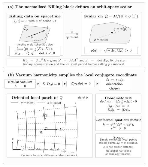
From orbit data to local Weyl coordinates. On a circular Lorentzian-orbit region, the normalized Killing Gram matrix defines $\rho^2=-\det\lambda$. Ricci-flat vacuum gives $D_h^2\rho=0$; after choosing the quotient orientation, $dz={*_h}d\rho$ makes the two coordinate gradients orthogonal and equal in norm, with nonzero Jacobian wherever $d\rho\ne0$. The diagram is schematic: it proves neither that $\rho$ is proper distance nor that the local chart extends to a global half-plane.

There are three different global questions that the local calculation does not answer:

1. A simply connected quotient makes the closed one-form ${*_h}d\rho$ globally exact, but it does not rule out critical points of $\rho$.
2. Even without critical points, the map $(\rho,z)$ still needs to be globally injective.
3. Identifying the image with a half-plane and its boundary with regular axes and horizons requires the global domain-of-outer-communications, asymptotic, topology, and boundary-regularity hypotheses of the black-hole uniqueness setting.

The local theorem is therefore powerful but modest: it constructs coordinates on regular patches; it is not by itself a global classification theorem. See Chruściel, Costa, and Heusler 2012, §§3.2.1–3.2.3, pp. 13–14 for the additional quotient and global qualifications.

Two Papapetrou parametrizations

The invariant statement is

$$ds^2=\lambda_{AB}\,dx^A dx^B +e^{2\nu}(d\rho^2+dz^2), \qquad \det\lambda=-\rho^2.$$

This matrix form remains meaningful whenever the Killing block is Lorentzian, including at a generic stationary-limit surface. Away from the rotation axis, set $X=g(\eta,\eta)>0$. An axial-norm parametrization is

$$ds^2=-\frac{\rho^2}{X}\,dt^2 +X(d\phi+W\,dt)^2 +e^{2\nu}(d\rho^2+dz^2).$$

Its Killing block has $g_{\phi\phi}=X$, $g_{t\phi}=XW$, and determinant $-\rho^2$ identically. This form is useful across a generic ergosurface because it is based on the axial norm rather than the stationary norm.

Only on a patch where $f=-g_{tt}>0$ should one pass to the familiar time-adapted form

$$ds^2=-f(dt-\omega\,d\phi)^2 +f^{-1}\left[e^{2\gamma}(d\rho^2+dz^2)+\rho^2d\phi^2\right],$$

where $\omega=g_{t\phi}/f$. Expanding again gives

$$g_{tt}=-f, \qquad g_{t\phi}=f\omega, \qquad g_{\phi\phi}=\frac{\rho^2}{f}-f\omega^2, \qquad \det\lambda=-\rho^2.$$

At a generic ergosurface $g_{tt}=0$ but $g_{t\phi}\ne0$, so

$$\rho=\lvert g_{t\phi}\rvert>0.$$

The ergosurface is therefore an interior curve of the orbit space, not part of the $\rho=0$ boundary. The metric and matrix form can remain regular while $\omega=g_{t\phi}/f$ diverges. This is a limitation of the time-adapted potentials, not a spacetime singularity; Chruściel, Costa, and Heusler 2012, §3.2.4, p. 15 discusses precisely this reduction issue. The metric function $\omega$ here should also not be confused with the twist one-form or the twist scalar introduced on the next page.

The vacuum equations now form a hierarchy. The determinant constraint and the matrix current govern the two independent entries of $\lambda$; in the $f,\omega$ chart these are the nonlinear dynamical equations. The remaining quotient equation determines $\nu$, or equivalently $\gamma$, by first-order quadratures. Twist and Ernst Potentials packages the dynamical pair into the Ernst equation.

The static Weyl subclass

If the selected stationary field is hypersurface orthogonal, take $\omega=0$ and write $f=e^{2U}$. The metric becomes

$$ds^2=-e^{2U}dt^2 +e^{-2U}\!\left[e^{2\gamma}(d\rho^2+dz^2)+\rho^2d\phi^2\right].$$

Vacuum first gives the axisymmetric Laplace equation on an auxiliary flat three-space,

$$\Delta_3U =U_{,\rho\rho}+\frac{1}{\rho}U_{,\rho}+U_{,zz}=0,$$

and then the quadratures

$$\gamma_{,\rho}=\rho\left(U_{,\rho}^2-U_{,z}^2\right), \qquad \gamma_{,z}=2\rho U_{,\rho}U_{,z}.$$

Do not confuse this equation $\Delta_3U=0$ with the earlier physical quotient equation $D_h^2\rho=0$: they act on different functions with different metrics. Exact differentiation of the quadratures gives

$$\partial_z\gamma_{,\rho}-\partial_\rho\gamma_{,z} =-2\rho U_{,z}\!\left( U_{,\rho\rho}+\frac{1}{\rho}U_{,\rho}+U_{,zz} \right).$$

The Laplace equation therefore guarantees compatibility. Compatibility alone is weaker on exceptional branches: $U=\rho$ and $\gamma=\rho^2/2$ satisfy both quadratures but $\Delta_3U=1/\rho\ne0$, so they do not solve the vacuum system. This is why the full field equation cannot be replaced by a bare curl test.

The linearity of $U$ is nevertheless enormously useful. One may superpose harmonic potentials, then compute the nonlinear metric function $\gamma$. The four-dimensional problem is not linear because $e^{2U}$ reconstructs the metric and $\gamma$ is quadratic in the gradients. These equations, with the minus sign in $\gamma_{,\rho}$, appear in Wald 1984, §7.1, Eqs. (7.1.26)–(7.1.29), pp. 167–168; see also Bičák 2000, §6.1, pp. 55–56, Eqs. (34)–(35).

An additive constant remains in $\gamma$. Once the period of $\phi$ is fixed to $2\pi$, it can enforce elementary flatness on one chosen connected axis interval. If the axis has several disconnected intervals, one constant need not regularize all of them; a mismatch represents a conical defect such as a strut.

Schwarzschild as an exact calibration

Let $m=GM_{\rm phys}>0$ in units $c=1$, and set $\Delta=r(r-2m)$. In the Schwarzschild exterior $r>2m$, $0<\theta<\pi$, define

$$\rho=\sqrt{r(r-2m)}\sin\theta, \qquad z=(r-m)\cos\theta.$$

The quotient metric before the Weyl transformation is

$$h=\frac{r^2}{\Delta}\,dr^2+r^2d\theta^2.$$

Direct calculation gives

$$D_h^2\rho=0, \qquad \frac{\partial(\rho,z)}{\partial(r,\theta)} =-\frac{\Delta+m^2\sin^2\theta}{\sqrt\Delta}\ne0,$$

and

$$d\rho^2+dz^2 =\left(\Delta+m^2\sin^2\theta\right) \left(\frac{dr^2}{\Delta}+d\theta^2\right).$$

With the coordinate orientation $dr\wedge d\theta$, the conventional choice of $z$ obeys $dz=-{*_h}d\rho$; reversing the quotient orientation gives the sign convention used above.

Introduce the Euclidean distances from the two endpoints of the finite boundary interval,

$$R_\pm=\sqrt{\rho^2+(z\pm m)^2}.$$

In the exterior they satisfy

$$R_\pm=r-m\pm m\cos\theta, \qquad R_++R_-=2(r-m).$$

The Weyl potentials reconstruct Schwarzschild exactly:

$$e^{2U}=\frac{R_++R_--2m}{R_++R_-+2m},$$ $$e^{2\gamma} =\frac{(R_++R_-)^2-4m^2}{4R_+R_-}.$$

The boundary preimages are equally instructive:

Spacetime set in the completed exterior	Orbit-space image	Degenerating Killing data
North axis: $\theta=0$, $r>2m$	$\rho=0$, $z>m$	axial field $\eta$ vanishes
Open horizon projection: $r=2m$, $0<\theta<\pi$	$\rho=0$, $-m<z<m$	horizon direction $\xi$ in Schwarzschild
South axis: $\theta=\pi$, $r>2m$	$\rho=0$, $z<-m$	axial field $\eta$ vanishes
Two pole–horizon corners	$(\rho,z)=(0,\pm m)$	the full Killing block tends to zero

Thus a smooth spherical horizon projects to an open line interval only after quotienting by time translations and rotations. The endpoints are separate rank-zero corner cases, not ordinary points of the horizon interval. The coordinate length $2m$ is not a proper horizon length. This finite interval is also a nondegenerate-horizon feature: in the extremal Kerr limit the horizon interval shrinks to a Weyl boundary point. Wald identifies the Schwarzschild finite rod in Wald 1984, §7.1, p. 168, while Bičák 2000, §6.1, pp. 55–56 gives the same Weyl-potential interpretation. The axis-structure page develops the interval kernels and endpoint regularity in detail.

What the assumptions are doing

The construction fails in informative ways when one removes a hypothesis.

Hypothesis	What it provides	What can fail without it
Two independent commuting symmetries	A rank-two orbit block and a two-dimensional quotient	No $2+2$ reduction
Circularity	Orthogonal orbit and meridional blocks	Mixed orbit–quotient terms remain
$\det\lambda<0$	A Lorentzian orbit plane and Riemannian quotient	The direct elliptic/Hodge construction changes type
Ricci-flat vacuum with $\Lambda=0$	$D_h^2\rho=0$	The determinant scalar can be sourced
$d\rho\ne0$	A nonzero $(\rho,z)$ Jacobian	Harmonic functions may have critical points
Suitable topology and boundary behavior	A global half-plane description	A local coordinate need not be global or injective

More generally, the orbit equations imply

$$D_h^2\rho=-\rho\,\lambda^{AB}R_{AB}, \qquad R_{AB}=R_{\mu\nu}K_A^\mu K_B^\nu.$$

Generic matter can therefore source $\rho$. Source-free, symmetry-inheriting Einstein–Maxwell theory with $\Lambda=0$ is an important exception: the relevant contraction vanishes and $\rho$ remains harmonic, as the Reissner–Nordström family confirms. A cosmological constant already changes the equation. For static (anti-)de Sitter with $F(r)=1-\Lambda r^2/3$ and $\rho=r\sqrt F\sin\theta$,

$$D_h^2\rho=-2\Lambda\rho.$$

Finally, $\rho=0$ should not be read as a universal synonym for “axis.” Depending on the completed quotient boundary, it can mark an axis interval, a nondegenerate horizon interval, or a corner; degenerate horizons can have a different Weyl image. The invariant block and the global hypotheses decide which interpretation is correct.

Common pitfalls

Treating $\rho$ as proper radius. It is the square root of minus a Gram determinant. Even in Schwarzschild, its level sets and scale differ from proper-distance circles.

Calling an ergosurface a Weyl boundary. At a generic stationary-limit surface, $f=0$ but $\rho=\lvert g_{t\phi}\rvert>0$. The time-adapted potential $\omega$ is singular there; the orbit matrix need not be.

Promoting a local conjugate to a global coordinate. Closedness gives $z$ locally, and simple connectedness removes periods. Neither statement rules out critical points or proves global injectivity.

Checking only the $\gamma$ curl. The vacuum Laplace equation guarantees the quadratures are compatible, but the converse has exceptional branches. The field equation for $U$ remains an independent requirement.

Exercises

1. Basis covariance

Let $K'_A=A_A{}^B K_B$ for a constant nonsingular matrix $A$. Derive the transformation laws for $\lambda$, $\rho$, and $z$. What happens for the shear $\xi'=\xi+\Omega\eta$, $\eta'=\eta$?

Solution

The Gram matrix transforms by congruence, $\lambda'=A\lambda A^{\mathsf T}$, so $\det\lambda'=(\det A)^2\det\lambda$ and $\rho'=\lvert\det A\rvert\rho$. With the same quotient orientation,

$$dz'={*_h}d\rho'=\lvert\det A\rvert\,dz,$$

so $z'=\lvert\det A\rvert z+C$. The shear has determinant one, hence leaves $\rho$ unchanged and changes $z$ only by an additive constant even though it changes the selected time flow.

2. The coordinate Jacobian

Starting from $dz={*_h}d\rho$ on an oriented Riemannian two-manifold, prove that $(\rho,z)$ is a coordinate system wherever $d\rho\ne0$.

Solution

For any one-form $\alpha$ in two-dimensional Riemannian geometry,

$$\alpha\wedge {*_h}\alpha =\lvert\alpha\rvert_h^2\operatorname{vol}_h.$$

Taking $\alpha=d\rho$ gives

$$d\rho\wedge dz =\lvert d\rho\rvert_h^2\operatorname{vol}_h.$$

The right-hand side is nonzero exactly when $d\rho\ne0$. The inverse-function theorem then makes $(\rho,z)$ a local chart. The same Hodge identity gives orthogonality and equal norms of the two gradients.

3. An ergosurface is not an orbit-space boundary

Expand the time-adapted Papapetrou metric, compute its Killing-block determinant, and show that a generic point with $g_{tt}=0$ and $g_{t\phi}\ne0$ has $\rho>0$.

Solution

The block entries are

$$g_{tt}=-f, \qquad g_{t\phi}=f\omega, \qquad g_{\phi\phi}=f^{-1}\rho^2-f\omega^2.$$

Therefore

$$g_{tt}g_{\phi\phi}-g_{t\phi}^2=-\rho^2.$$

At a generic stationary-limit point, direct use of the invariant determinant gives $\det\lambda=-g_{t\phi}^2$, hence $\rho=\lvert g_{t\phi}\rvert>0$. The displayed $f,\omega$ chart is singular because $\omega=g_{t\phi}/f$, but the orbit matrix has full rank and the point lies in the quotient interior.

4. Why the curl test is weaker

Derive the exact compatibility identity for the static $\gamma$ quadratures. Then test $U=\rho$ and $\gamma=\rho^2/2$.

Solution

Differentiate the first quadrature with respect to $z$ and the second with respect to $\rho$. After canceling the mixed-derivative terms,

$$\partial_z\gamma_{,\rho}-\partial_\rho\gamma_{,z} =-2\rho U_{,z}\Delta_3U.$$

For $U=\rho$, the proposed $\gamma$ has $\gamma_{,\rho}=\rho$ and $\gamma_{,z}=0$, so both quadratures hold and their curl vanishes. But $\Delta_3U=1/\rho$, not zero. The pair is therefore compatible without being a vacuum Weyl solution.

5. Reconstruct Schwarzschild

Using the Schwarzschild map, prove the identities for $R_\pm$ and recover $e^{2U}=1-2m/r$. Then identify the three open pieces of the completed $\rho=0$ boundary.

Solution

Substitution gives

$$R_\pm^2 =r(r-2m)\sin^2\theta+\bigl((r-m)\cos\theta\pm m\bigr)^2 =\bigl(r-m\pm m\cos\theta\bigr)^2.$$

The exterior inequalities make the positive square roots

$$R_\pm=r-m\pm m\cos\theta.$$

Hence $R_++R_-=2(r-m)$ and

$$e^{2U} =\frac{2(r-m)-2m}{2(r-m)+2m} =1-\frac{2m}{r}.$$

For $\theta=0$ and $r>2m$, one obtains $z=r-m>m$; for $\theta=\pi$, $z=-(r-m)<-m$; and for $r=2m$, $0<\theta<\pi$, one obtains $z=m\cos\theta\in(-m,m)$. These are respectively the north axis, south axis, and open horizon projection. The values $z=\pm m$ are the two separate corner limits.

References

• Bičák, Jiří. “Selected Solutions of Einstein’s Field Equations: Their Role in General Relativity and Astrophysics.” In Einstein’s Field Equations and Their Physical Implications, Lecture Notes in Physics 540, 1–126. Springer, 2000. DOI: 10.1007/3-540-46580-4_1. Open PDF.
• Chruściel, Piotr T., João Lopes Costa, and Markus Heusler. “Stationary Black Holes: Uniqueness and Beyond.” Living Reviews in Relativity 15 (2012): 7. DOI: 10.12942/lrr-2012-7.
• Wald, Robert M. General Relativity. Chicago: University of Chicago Press, 1984. ISBN 978-0-226-87033-5. Publisher record.