Twist and Ernst Potentials

The Killing norm and a locally defined twist potential form the two scalar fields in the stationary vacuum reduction. On a timelike Ricci-flat patch, they combine into a complex Ernst potential $\mathcal E=f+i\chi$. One nonlinear equation then carries the norm and rotation equations together—but it does not by itself supply the reconstructed metric, a regular axis, a horizon extension, or the global topology.

Required background. Killing Fields and Isometry Groups supplies Killing reduction; The Einstein Equation supplies the vacuum and electrovac identities.

Helpful background. The Riemann Curvature Tensor supplies the twist-closure identity; Formulations of General Relativity supplies reduced actions; Causality and Global Structure supplies the topology needed for global potentials.

The full twist of a stationary Killing field

Let $\xi$ be the stationary Killing field. When an asymptotically flat end is available, normalize it there so that $\xi^2\to-1$. The symbol $\xi^\flat$ denotes the one-form metric-dual to $\xi$. With the site orientation $\epsilon_{tr\theta\phi}=+\sqrt{-g}$, the Lorentzian Hodge dual of a $p$-form $\alpha$ is fixed by

$$(*\alpha)_{\mu_{p+1}\ldots\mu_4} =\frac{1}{p!}\alpha^{\mu_1\ldots\mu_p} \epsilon_{\mu_1\ldots\mu_4}.$$

Define the norm and full twist one-form by

$$f=-\xi^\mu\xi_\mu, \qquad \varpi=-{*}\!\left(\xi^\flat\wedge d\xi^\flat\right),$$

or, in components,

$$\varpi_\mu=\epsilon_{\mu\nu\rho\sigma} \xi^\nu\nabla^\rho\xi^\sigma.$$

The minus sign in the form expression follows from placing the three contracted indices before the output index in the Hodge convention above; it makes the displayed component formula the primary sign definition. The symbol $\varpi$ prevents confusion with the Papapetrou shift used on the preceding Weyl–Papapetrou page. Some references absorb this sign into their Hodge convention or call $\tfrac12\varpi$ the twist, so comparisons must begin with the definitions.

The Killing identity gives the four-dimensional relation

$$d\varpi=-2{*}\!\left(\xi^\flat\wedge R(\xi)\right), \qquad R(\xi)_\mu=R_{\mu\nu}\xi^\nu.$$

It follows that $d\varpi=0$ in Ricci-flat vacuum. Closure also survives an Einstein space $R_{\mu\nu}=\Lambda g_{\mu\nu}$ because the wedge then contains $\xi^\flat$ twice, although the Ricci-flat Ernst equation below does not survive unchanged. The sign also agrees with the circularity page: its form-defined twist is $\tau=*(\xi^\flat\wedge d\xi^\flat)=-\varpi$, so $d\tau=+2*(\xi^\flat\wedge R(\xi))$. Chruściel, Costa, and Heusler give the corresponding curvature identity for their half twist in CCH 2012, §8.1, printed p. 42, Eq. (8.1). Translating that definition together with the Hodge convention, rather than only doubling the twist, gives the identity above. Their half-twist definition and timelike reduction appear in §§6.1–6.2, printed pp. 31–33.

Locally, the Poincaré lemma now supplies a real scalar $\chi$ such that

$$d\chi=\varpi.$$

Globally, this requires every period $\oint_C\varpi$ to vanish; simple connectedness is a sufficient, not necessary, condition. The value of $\chi$ is gauge-dependent because $\chi\mapsto\chi+c$ changes no geometry. Wherever $\xi\ne0$, $\varpi=0$ is equivalent to hypersurface orthogonality of this chosen Killing field. It yields local staticity where $\xi$ is timelike. Thus $d\chi$, not a nonzero value of $\chi$, diagnoses vacuum twist; global staticity needs additional completeness and topology.

These four-dimensional statements need no assumption that $\xi$ is timelike. The restriction $f>0$ enters in the next step, where the quotient becomes Riemannian. A smooth twist potential may cross a stationary-limit surface even though the timelike reduction fails there.

Timelike reduction and the Ernst equation

For this section assume $R_{\mu\nu}=0$ and restrict to a connected region with $f>0$. The tensor

$$q_{\mu\nu}=f g_{\mu\nu}+\xi_\mu\xi_\nu$$

annihilates $\xi$ and is therefore degenerate as a four-dimensional tensor. Its pullback to any local section, equivalently its descent to the three-dimensional orbit space $\mathcal B$, is positive definite. Let $D$ be its Levi–Civita derivative, $D^2=D_iD^i$, and let the centered dot denote contraction with $q^{ij}$.

After writing the stationary metric locally as

$$g=-f(dt-A)^2+f^{-1}q,$$

the one-form $A$ carries the stationary off-diagonal, or frame-dragging, data. Its vacuum field equation says that $f^2{*_q}dA$ is locally closed, so on the same potential patch it equals $d\chi$. Working per unit interval of the Killing parameter and discarding a boundary term, the Einstein–Hilbert action reduces to

$$S_{\mathrm{red}}\propto \int_{\mathcal B}\!\sqrt q\,d^3x \left[ R(q)-\frac{Df\!\cdot Df+D\chi\!\cdot D\chi}{2f^2} \right].$$

The scalar part is a harmonic-map energy with target metric

$$ds_{\mathcal T}^2=\frac{df^2+d\chi^2}{2f^2}, \qquad f>0.$$

Varying $f$ and $\chi$ gives

$$D^2f=f^{-1}\!\left(Df\!\cdot Df-D\chi\!\cdot D\chi\right), \qquad D^2\chi=2f^{-1}Df\!\cdot D\chi.$$

Now define

$$\mathcal E=f+i\chi.$$

Since $\operatorname{Re}\mathcal E=f$, the two real equations are exactly the real and imaginary parts of

$$(\operatorname{Re}\mathcal E)D^2\mathcal E =D\mathcal E\!\cdot D\mathcal E.$$

This is the vacuum Ernst equation. It is nonlinear because the target is curved, not because the complex field introduces an extra degree of freedom. The three-dimensional Einstein equation still determines the quotient metric,

$$R_{ij}(q)=\frac{1}{2f^2} \left(D_i fD_j f+D_i\chi D_j\chi\right).$$

So the complex equation is the dynamical core of the reduction, not the whole four-dimensional solution. The action, target geometry, and field equations are derived in Chruściel, Costa, and Heusler 2012, §§6.1–6.2, printed pp. 31–33.

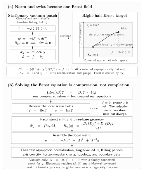
Vacuum Ernst reduction and reconstruction. On a simply connected timelike Ricci-flat patch, $\mathcal E=f+i\chi$ maps the orbit space into the right half-plane with target metric $(df^2+d\chi^2)/(2f^2)$. After fixing $\chi\to0$ at the selected infinity, static data lie on $\chi=0$; invariant rotation is carried by $d\chi$. Solving the Ernst equation yields $(f,\chi)$, but the shift $A$, quotient metric $q$ or Weyl factor $\gamma$, periods, axes, horizons, topology, and boundary data remain to be reconstructed and checked. The diagram is schematic, vacuum-only, and not an orbit-space or spacetime embedding; $f=0$ ends this timelike reduction but is not automatically a curvature singularity.

Axisymmetry and metric reconstruction

Now also assume circular axial symmetry and work on a Weyl patch with $\rho>0$. With $\phi\sim\phi+2\pi$ and all potentials independent of $\phi$,

$$q=e^{2\gamma}(d\rho^2+dz^2)+\rho^2d\phi^2.$$

For any two axisymmetric scalars $s$ and $u$,

$$D^2s=e^{-2\gamma} \left(s_{,\rho\rho}+\rho^{-1}s_{,\rho}+s_{,zz}\right), \qquad Ds\!\cdot Du=e^{-2\gamma} \left(s_{,\rho}u_{,\rho}+s_{,z}u_{,z}\right).$$

The common conformal factor cancels. Writing

$$\Delta_3=\partial_\rho^2+\rho^{-1}\partial_\rho+\partial_z^2,$$

the Ernst equation becomes

$$(\operatorname{Re}\mathcal E)\Delta_3\mathcal E =\mathcal E_{,\rho}^2+\mathcal E_{,z}^2.$$

The apparent $\rho^{-1}$ singularity is the ordinary cylindrical Laplacian. On a regular axis it is interpreted by smooth even extension in the local Cartesian coordinates, not by deleting the axis term.

To see exactly what remains, take $A=\Omega(\rho,z)d\phi$ and orient $q$ by $d\rho\wedge dz\wedge d\phi$. The three-dimensional star $*_q$ uses the same component convention as above with the Riemannian volume form of $q$. With the standard Weyl choice inherited from the preceding page, the site orientation has $\epsilon_{t\rho z\phi}=-\sqrt{-g}$; this relative orientation is what fixes the plus sign in $d\chi=f^2{*_q}dA$. Its components are

$$\Omega_{,\rho}=-\rho f^{-2}\chi_{,z}, \qquad \Omega_{,z}=\rho f^{-2}\chi_{,\rho}.$$

The quotient equation supplies

$$\gamma_{,\rho}=\frac{\rho}{4f^2} \left(f_{,\rho}^2-f_{,z}^2+\chi_{,\rho}^2-\chi_{,z}^2\right),$$ $$\gamma_{,z}=\frac{\rho}{2f^2} \left(f_{,\rho}f_{,z}+\chi_{,\rho}\chi_{,z}\right).$$

The Ernst equation makes these first-order systems locally compatible, but global integration can still fail through nonzero periods. Each connected integration domain has one overall additive constant for $\gamma$: normalize one regular axis segment, then test the others. Incompatible conicities signal a physical strut or string, not extra freedom to choose a different constant on every segment. Bičák gives this hierarchy in Bičák 2000, §§6.2–6.3, printed pp. 58–60, Eqs. (36)–(39), Open PDF; his $g=-f(dt+A_{\mathrm B}d\phi)^2+\cdots$ maps to the present convention by $\Omega=-A_{\mathrm B}$. The $\gamma$ equations can be checked directly against Griffiths and Podolský 2009, §13.2.1, printed p. 247, Eq. (13.12), and the original complex formulation is in Ernst 1968, Part I, pp. 1175–1178.

Static and rotating calibrations

The static branch is an immediate sign and factor check. In this subsection, $\nabla$ is the flat cylindrical gradient in $(\rho,z)$ and $\nabla^2=\Delta_3$. If $d\chi=0$, choose the additive gauge $\chi=0$ and write $\mathcal E=f=e^{2U}$. Substitution gives

$$e^{4U}\left(2\Delta_3U+4\nabla U\!\cdot\nabla U\right) =4e^{4U}\nabla U\!\cdot\nabla U,$$

so

$$\Delta_3U=0.$$

The Weyl–Papapetrou page works through the Schwarzschild rod potential and its horizon interpretation. Here the more discriminating calibration is Kerr. Write $m=GM_{\mathrm{phys}}$ and $a=J_{\mathrm{phys}}/M_{\mathrm{phys}}$ in $c=1$ units, and use $j=GJ_{\mathrm{phys}}=ma$ for the geometrized angular momentum. Set

$$\Sigma=r^2+a^2\cos^2\theta, \qquad j=ma.$$

For the site orientation and $\xi=\partial_t$ normalized at infinity,

$$\mathcal E_{\mathrm{Kerr}} =1-\frac{2m}{r-ia\cos\theta},$$

and therefore

$$f=1-\frac{2mr}{\Sigma}, \qquad \chi=-\frac{2ma\cos\theta}{\Sigma}.$$

At large $r$,

$$\mathcal E =1-\frac{2m}{r}-\frac{2ij\cos\theta}{r^2}+O(r^{-3}).$$

The real monopole fixes the mass normalization; the leading odd-parity imaginary term fixes the signed angular momentum. Sending $a\to0$ recovers Schwarzschild and $\chi=0$. Reversing the spacetime orientation reverses the Hodge dual and hence the sign of $\chi$. The scalar expression remains finite at a generic Kerr stationary-limit surface $f=0$, while the positive timelike quotient and its elliptic interpretation end there. This cleanly separates failure of reduced variables from a four-dimensional singularity. The convention-translated Kerr field is recorded in Griffiths and Podolský 2009, §13.2.2, printed pp. 249–250. The next page turns the asymptotic coefficients into properly normalized relativistic multipole moments.

Einstein–Maxwell: the corrected twist

For electrovac, conventions are part of the equation. Use $\Lambda=0$ and the geometrized field $\widehat F$ in

$$S=\frac{1}{16\pi G}\int d^4x\sqrt{-g} \left(R-\widehat F_{\mu\nu}\widehat F^{\mu\nu}\right).$$

If $F_{\mathrm{phys}}$ is a Gaussian-normalized physical field, then $\widehat F=\sqrt G\,F_{\mathrm{phys}}$. A charge parameter $Q$ appearing in the metric has dimensions of length and obeys $Q^2=GQ_{\mathrm{phys}}^2$ for a purely electric solution.

Assume $\mathcal L_\xi\widehat F=0$ and the source-free Maxwell equations. Here $i_\xi$ denotes interior contraction with the Killing field: $(i_\xi\widehat F)_\mu=\xi^\nu\widehat F_{\nu\mu}$. Cartan’s identity then makes the one-forms below closed, so locally define

$$d\varphi=-i_\xi\widehat F, \qquad d\psi=i_\xi{*\widehat F}, \qquad \Phi=\varphi+i\psi.$$

The differential-form formulation of electromagnetism develops the closure step and the role of the Hodge dual in detail.

Electromagnetic momentum sources the raw gravitational twist. With the declared Hodge orientation, the locally closed combination is

$$d\chi =\varpi-2\left(\varphi\,d\psi-\psi\,d\varphi\right) =\varpi-2\operatorname{Im}(\bar\Phi\,d\Phi).$$

This $\chi$ is a generalized twist potential. Define

$$\mathcal E=f-\lvert\Phi\rvert^2+i\chi, \qquad f=\operatorname{Re}\mathcal E+\lvert\Phi\rvert^2.$$

The definitions are designed so that the convention-sensitive pieces collapse into the simple current

$$P:=d\mathcal E+2\bar\Phi\,d\Phi =df+i\varpi.$$

On the timelike quotient, the coupled Ernst equations are

$$fD^2\mathcal E=P\!\cdot D\mathcal E, \qquad fD^2\Phi=P\!\cdot D\Phi.$$

On a circular Weyl patch the same conformal-factor cancellation replaces $D^2$ and the dot product by $\Delta_3$ and the flat cylindrical dot product. Setting $\Phi=0$ recovers vacuum. Setting $d\chi=0$ does not by itself imply staticity, because the electromagnetic bilinear can cancel the raw twist; local staticity of the selected timelike field remains $\varpi=0$. To reconstruct the shift, first recover the raw twist as $\varpi=d\chi+2\operatorname{Im}(\bar\Phi\,d\Phi)$ and substitute it for $d\chi$ in the vacuum shift relation; the quotient-metric equations likewise acquire electromagnetic terms. The directly inspected reduction is in Chruściel, Costa, and Heusler 2012, §6.4, printed pp. 34–36, Eqs. (6.19)–(6.26), after translating its half-twist and Hodge conventions. The stationary-axisymmetric equations and reconstruction appear in Griffiths and Podolský 2009, §§13.2.1–13.3.1, printed pp. 246–254.

The exact benchmark table fixes the normalization. Here $\widehat F=d\widehat{\mathcal A}$, and the gauge potential is $\widehat{\mathcal A}=-Q\,dt/r$ in the charged static row.

Family	$\mathcal E$	$\Phi$	Recovered $f$
Minkowski	$1$	$0$	$1$
Schwarzschild	$1-2m/r$	$0$	$1-2m/r$
Kerr	$1-2m/(r-ia\cos\theta)$	$0$	$1-2mr/\Sigma$
Reissner–Nordström	$1-2m/r$	$-Q/r$	$1-2m/r+Q^2/r^2$
Kerr–Newman	$1-2m/(r-ia\cos\theta)$	$-Q/(r-ia\cos\theta)$	$1-(2mr-Q^2)/\Sigma$

Reissner–Nordström makes the key point especially clearly: in electrovac, $\operatorname{Re}\mathcal E$ is not the Killing norm $f$ by itself. The missing $Q^2/r^2$ comes from $\lvert\Phi\rvert^2$. Kerr–Newman independently fixes the magnetic-potential and generalized-twist signs: differentiating its four-metric and Maxwell field with $\epsilon_{tr\theta\phi}=+\sqrt{-g}$ gives $\psi=-Qa\cos\theta/\Sigma$ and the displayed $d\chi$ relation. The convention-translated charged benchmarks are supported by Griffiths and Podolský 2009, §13.3.2, printed pp. 254–255.

Gauge, normalization, and what remains physical

The electric and magnetic zero points are coupled to the generalized twist gauge. For a constant $\beta\in\mathbb C$ and real $c$,

$$\Phi'=\Phi+\beta,$$ $$\mathcal E' =\mathcal E-2\bar\beta\Phi-\lvert\beta\rvert^2+ic.$$

Then $f'=f$ and

$$d\mathcal E'+2\bar\Phi' d\Phi' =d\mathcal E+2\bar\Phi d\Phi.$$

Writing $\beta=\beta_e+i\beta_m$ shows explicitly that $\varphi\mapsto\varphi+\beta_e$ and $\psi\mapsto\psi+\beta_m$ require

$$\chi\mapsto\chi-2\beta_e\psi+2\beta_m\varphi+c.$$

The three additive constants are therefore not independent once $(\mathcal E,\Phi)$ is used. Separately, rescaling the Killing field by a nonzero constant $s$ sends the zero-gauge representatives as

$$f\mapsto s^2f, \qquad \Phi\mapsto s\Phi, \qquad \chi\mapsto s^2\chi, \qquad \mathcal E\mapsto s^2\mathcal E.$$

Fix the stationary generator and all potential zero points at the selected asymptotic end before comparing formulas or reading mass, spin, and charge. The later Ehlers and Harrison transformations act precisely on these reduced potentials, while Verifying and Interpreting Generated Solutions explains why reduced equations, reconstruction, global identifications, and physical admissibility are separate gates.

Common pitfalls

Reading rotation from the value of $\chi$. An additive constant can make a nonzero constant vanish or a zero constant nonzero. In vacuum the invariant local statement is $d\chi=\varpi$; in electrovac one must recover $\varpi=d\chi+2\operatorname{Im}(\bar\Phi d\Phi)$.

Treating $f=0$ as a curvature singularity. It is where the chosen stationary Killing field becomes null and the positive timelike quotient degenerates. Kerr’s generic ergosurface is smooth and lies at $\rho>0$ in the invariant two-Killing orbit space.

Stopping after the complex PDE. The shift, quotient metric, integration constants, periods, axis conicity, boundary data, and horizon-regular extension remain. A local Ernst solution is not yet a globally admissible spacetime.

Mixing electrovac conventions. Reversing orientation, changing the Hodge-star sign, using a half-twist, or omitting the $\sqrt G$ conversion changes the printed potentials. Translate the complete set $(\widehat F,\varpi,\Phi,\chi,\mathcal E)$ before borrowing a formula.

Exercises

1. Recover both real vacuum equations

Show directly that the real and imaginary parts of the vacuum Ernst equation reproduce the two scalar equations for $f$ and $\chi$.

Solution

Insert $\mathcal E=f+i\chi$. Then

$$D\mathcal E\!\cdot D\mathcal E =Df\!\cdot Df-D\chi\!\cdot D\chi +2iDf\!\cdot D\chi.$$

Because $\operatorname{Re}\mathcal E=f$, equating real and imaginary parts of $fD^2\mathcal E=D\mathcal E\cdot D\mathcal E$ gives

$$D^2f=f^{-1}\left(Df\!\cdot Df-D\chi\!\cdot D\chi\right),$$ $$D^2\chi=2f^{-1}Df\!\cdot D\chi.$$

2. Closed need not mean globally exact

On the punctured plane $\mathbb R^2\setminus\{0\}$, consider

$$\alpha=\frac{-y\,dx+x\,dy}{x^2+y^2}.$$

Show that $d\alpha=0$ but that no single-valued global scalar $u$ satisfies $du=\alpha$.

Solution

Direct differentiation gives $d\alpha=0$ away from the origin. On the unit circle $x=\cos\vartheta$, $y=\sin\vartheta$, one has $\alpha=d\vartheta$, so

$$\oint_{S^1}\alpha=2\pi.$$

The integral of an exact one-form around a closed curve would vanish. Thus $\alpha$ is locally $d\vartheta$ but has no global single-valued potential. The same distinction separates local twist potentials from a global $\chi$ on a nonsimply connected orbit domain.

3. Why the static branch becomes Laplace’s equation

Set $\mathcal E=e^{2U}$ with real $U$ and derive the axisymmetric Laplace equation.

Solution

The chain rule gives

$$\Delta_3\mathcal E =2e^{2U}\Delta_3U+4e^{2U}\nabla U\!\cdot\nabla U,$$ $$\nabla\mathcal E\!\cdot\nabla\mathcal E =4e^{4U}\nabla U\!\cdot\nabla U.$$

Multiplying the first line by $\operatorname{Re}\mathcal E=e^{2U}$ and comparing with the second cancels the gradient-square terms, leaving $2e^{4U}\Delta_3U=0$. Hence $\Delta_3U=0$ wherever $f=e^{2U}>0$.

4. Read mass and spin from Kerr

Starting from

$$\mathcal E=1-\frac{2m}{r-ia\cos\theta},$$

find $f$, $\chi$, the first two asymptotic orders, and the $a\to0$ limit.

Solution

Multiply by the complex conjugate denominator:

$$\frac{1}{r-ia\cos\theta} =\frac{r+ia\cos\theta}{\Sigma}.$$

Therefore

$$f=1-\frac{2mr}{\Sigma}, \qquad \chi=-\frac{2ma\cos\theta}{\Sigma}.$$

Expanding the reciprocal gives

$$\mathcal E =1-\frac{2m}{r}-\frac{2ima\cos\theta}{r^2}+O(r^{-3}).$$

Thus the mass length is $m$ and the signed geometrized angular momentum is $j=ma=GJ_{\mathrm{phys}}$. Restoring physical units gives $J_{\mathrm{phys}}=ma/G$ when $c=1$. At $a=0$, $\Sigma=r^2$, $\chi=0$, and $\mathcal E=1-2m/r$, the Schwarzschild result.

5. Why electrovac needs two complex potentials

On a connected Reissner–Nordström region where the stationary field is timelike, so $f>0$—for example, the exterior $r>r_+$ of a subextremal black hole with $m^2>Q^2$ and $r_+=m+\sqrt{m^2-Q^2}$—take

$$\mathcal E=1-\frac{2m}{r}, \qquad \Phi=-\frac{Q}{r}.$$

Recover $f$, and verify the radial coupled Ernst equations using

$$q=dr^2+fr^2d\Omega_2^2.$$

Solution

First,

$$f=\operatorname{Re}\mathcal E+\lvert\Phi\rvert^2 =1-\frac{2m}{r}+\frac{Q^2}{r^2}.$$

For a radial scalar $s$,

$$D^2s=\frac{1}{fr^2}\frac{d}{dr} \left(fr^2\frac{ds}{dr}\right).$$

Because this benchmark has a real electromagnetic potential, $\bar\Phi=\Phi$. The radial current is therefore

$$P_r=\mathcal E'+2\Phi\Phi'=f'.$$

Since $\mathcal E'=2m/r^2$,

$$fD^2\mathcal E =\frac{1}{r^2}\frac{d}{dr}(fr^2\mathcal E') =f'\mathcal E'=P_r\mathcal E'.$$

Likewise, $\Phi'=Q/r^2$ and

$$fD^2\Phi =\frac{1}{r^2}\frac{d}{dr}(fr^2\Phi') =f'\Phi'=P_r\Phi'.$$

The same $\mathcal E$ as Schwarzschild therefore does not imply the same metric: $\Phi$ supplies the charge term in $f$ and satisfies its own coupled equation.

References

• Bičák, Jiří. “Selected Solutions of Einstein’s Field Equations: Their Role in General Relativity and Astrophysics.” In Einstein’s Field Equations and Their Physical Implications: Selected Essays in Honour of Jürgen Ehlers, edited by Bernd G. Schmidt, 1–126. Lecture Notes in Physics 540. Berlin and Heidelberg: Springer, 2000. DOI. Open PDF.
• Chruściel, Piotr T., João Lopes Costa, and Markus Heusler. “Stationary Black Holes: Uniqueness and Beyond.” Living Reviews in Relativity 15, 7 (2012). DOI. Open PDF.
• Ernst, Frederick J. “New Formulation of the Axially Symmetric Gravitational Field Problem. I.” Physical Review 167, no. 5 (1968): 1175–1178. DOI.
• Ernst, Frederick J. “New Formulation of the Axially Symmetric Gravitational Field Problem. II.” Physical Review 168, no. 5 (1968): 1415–1417; erratum, Physical Review 172 (1968): 1850. Article DOI. Erratum DOI.
• Griffiths, Jerry B., and Jiří Podolský. Exact Space-Times in Einstein’s General Relativity. Cambridge Monographs on Mathematical Physics. Cambridge: Cambridge University Press, 2009. DOI.