Ergoregions, Killing Horizons, and Axis Structure

Orbit-space data distinguish three different ways a preferred Killing field can degenerate: the stationary field can become null on a stationary-limit surface, a linear combination of stationary and axial fields can generate a Killing horizon, or the axial field can vanish on a rotation axis. All may occur where a simple coordinate expression changes character, but their invariant tests and regularity conditions are different.

Required background. Killing Fields and Isometry Groups supplies Killing horizons and fixed sets; The Einstein Equation supplies the reduced stationary constraints.

Helpful background. The Riemann Curvature Tensor supports regularity checks; Formulations of General Relativity supplies quotient data; Causality and Global Structure supplies event-horizon and causal-boundary distinctions.

Stationary regions and ergoregions

Fix the stationary Killing field $\xi$ by unit normalization at an asymptotically flat end, and specify the domain of outer communications associated with that end. Its stationary region is where

$$g(\xi,\xi)<0.$$

On this page, an ergoregion is a connected part of that chosen exterior where $g(\xi,\xi)>0$, so no observer following the stationary flow can have a timelike worldline. Its boundary in the exterior, where $g(\xi,\xi)=0$, is a stationary-limit surface. The exterior qualifier matters: in maximally extended Schwarzschild, $\xi=\partial_t$ is spacelike for $r<2GM$, but the Schwarzschild domain of outer communications has no ergoregion. This definition also depends on the physically selected asymptotic time translation; an arbitrary helical Killing field in flat spacetime becomes null at a light cylinder, which is not a black-hole horizon.

A stationary-limit surface need not be null as a hypersurface. Its normal is $\nabla_\mu[g(\xi,\xi)]$, whereas the null vector $\xi$ is tangent to the symmetry flow. Only special geometric relations make the two align. In Kerr with $a\ne0$, the outer stationary-limit surface meets the horizon at the poles but lies outside it elsewhere. At the Schwarzschild endpoint $a=0$, the two loci coincide at every angle and the ergoregion disappears.

Killing horizons from the Gram matrix

Let $K_A=(\xi,\eta)$ and $\lambda_{AB}=g(K_A,K_B)$. Where

$$\rho^2=-\det\lambda=0,$$

the Killing block is singular. On a regular interval interior its kernel is one-dimensional and has a nonzero coefficient vector $v^A$. On a horizon interval of a circular stationary black hole, that kernel selects the combination

$$\chi=v^A K_A=\xi+\Omega_H\eta$$

as the candidate horizon generator.

On either the future or past horizon branch away from a bifurcation surface, $\chi$ is nonzero, null, and normal to the null hypersurface. At a bifurcation surface the same Killing field vanishes; the interval label still records the limiting projective kernel direction. For a connected regular horizon in the usual Einstein–Maxwell setting, $\Omega_H$ is constant. Its value changes if the basis $(\xi,\eta)$ is renormalized, which is why asymptotic time and the axial period were fixed first.

The local condition $\det\lambda=0$ alone does not prove that the set is a horizon. One must verify that the degenerating combination is null and normal to a smooth null hypersurface, then use global information before calling it an event horizon. The black-hole geometry volume develops general horizon mechanics, generator normalization, and surface gravity.

Axes, intervals, and conical regularity

On an axis interval, the kernel vector instead selects the periodic generator $\eta$, and $\eta$ vanishes at the fixed set. With $X=g(\eta,\eta)$ and period $2\pi$, elementary flatness requires

$$\lim_{X\to0}\frac{\nabla_\mu X\nabla^\mu X}{4X}=1.$$

If the limit is $\alpha^2\ne1$, the local circumference-to-radius ratio is $2\pi\alpha$ and a conical deficit or excess remains. Rescaling $\phi$ can regularize one connected axis segment but may spoil another because the angular period is a single global choice. This fact is central for accelerating solutions.

For many circular black-hole exteriors, the Weyl orbit space is a half-plane. Its $\rho=0$ boundary decomposes into ordered open intervals labeled by their degenerating Killing combination: axis intervals carry the axial label, and horizon intervals carry $\xi+\Omega_H\eta$. At an endpoint, the incident interval labels have well-defined one-sided limits, but the endpoint kernel itself can be higher-dimensional and need not select one unique direction. Chruściel, Costa, and Heusler explain the four-dimensional orbit-space structure in Chruściel, Costa, and Heusler 2012, §§3.2.1 and 3.2.3, printed pp. 13–14; the projective interval-direction description is developed in Harmark 2004, §§3.1–3.3, printed pp. 9–15.

In four dimensions with one axial field the labels are simple; in higher dimensions several axial generators can degenerate in different integer combinations. Even in four dimensions, an interval diagram records symmetry degeneration, not the full causal geometry or metric.

Schwarzschild calibration

For Schwarzschild with $m=GM>0$, choose $\xi=\partial_t$ and $\eta=\partial_\phi$. In the exterior,

$$\lambda =\begin{pmatrix} -(1-2m/r) & 0\\ 0 & r^2\sin^2\theta \end{pmatrix},$$

so the Weyl coordinates may be taken as

$$\rho=\sqrt{r(r-2m)}\,\sin\theta, \qquad z=(r-m)\cos\theta.$$

The open orbit-space region $r>2m$, $0<\theta<\pi$ has $\rho>0$. Its completed $\rho=0$ boundary separates into three interval interiors:

• On $\theta=\pi$, $r>2m$, one has $z<-m$ and $\ker\lambda=\operatorname{span}\{\eta\}$.
• On $r=2m$, $0<\theta<\pi$, one has $-m<z<m$ and $\ker\lambda=\operatorname{span}\{\xi\}$, with $\Omega_H=0$.
• On $\theta=0$, $r>2m$, one has $z>m$ and $\ker\lambda=\operatorname{span}\{\eta\}$.

At $z=\pm m$, both diagonal entries vanish, so $\lambda=0_{2\times2}$ and $\dim\ker\lambda=2$. The endpoint therefore does not determine a unique interval direction by itself. The finite timelike rod flanked by two axial rods is the Schwarzschild source diagram of Emparan and Reall 2002, §3.2, printed pp. 11–12, Fig. 2(a), PDF.

The figure makes the distinction geometrically explicit. Read its labels on the open interval interiors; the diamond endpoints are a separate kernel-rank case.

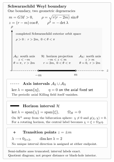
For the Schwarzschild exterior with $m=GM>0$, $\rho=\sqrt{r(r-2m)}\sin\theta$ and $z=(r-m)\cos\theta$ map $r>2m$ to $\rho>0$. The completed $\rho=0$ boundary consists of the south axis $z<-m$ with $\ker\lambda=\operatorname{span}\{\eta\}$, the horizon interval $-m<z<m$ with $\ker\lambda=\operatorname{span}\{\xi\}$ and $\Omega_H=0$, and the north axis $z>m$ with the axial kernel again. On the future and past horizon branches away from the bifurcation sphere, $\chi=\xi$ is nonzero and null; on the bifurcation sphere it vanishes. At $z=\pm m$, $\lambda\to0_{2\times2}$ and $\dim\ker\lambda=2$, so no single interval direction is selected by the endpoint kernel. The semi-infinite axes are truncated, and the quotient diagram shows neither proper distance nor the black-hole interior.

A practical discrimination sequence

Given a stationary-axisymmetric metric, first normalize $\xi$ and the period of $\eta$. Compute $g(\xi,\xi)$ to locate stationary limits. Next compute $\lambda_{AB}$ and its kernel on $\det\lambda=0$. If the kernel is the vanishing periodic field, test elementary flatness; if it is a nonzero null combination, test hypersurface normality and regular extension. Finally inspect curvature invariants and the global domain. This order prevents three common errors: calling every $g_{tt}=0$ surface a horizon, calling every $\rho=0$ interval an axis, and treating a conical defect as a coordinate artifact.

Exercises

Suppose the Killing block on a boundary interval has kernel generated by $(1,\Omega)$, while neither $\xi$ nor $\eta$ vanishes. What must still be checked before calling the interval a black-hole horizon?

Solution

Form $\chi=\xi+\Omega\eta$. One must show that the boundary lifts to a smooth null hypersurface, that $\chi$ is nonzero on each horizon branch away from any bifurcation surface and is normal as well as tangent there, and that a regular chart crosses it. At a bifurcation surface $\chi$ may vanish, so nonvanishing is not imposed there. Constancy and normalization of $\Omega$ must be controlled. Calling it an event horizon further requires the global causal relation to the chosen asymptotic end; the Gram matrix alone establishes none of those global facts.

Starting from the Schwarzschild Killing block above, derive all three open $\rho=0$ intervals and show explicitly why neither endpoint has a unique kernel direction.

Solution

Because

$$\rho^2=-\det\lambda=r(r-2m)\sin^2\theta,$$

the exterior boundary $\rho=0$ occurs either at $\theta=0$, at $\theta=\pi$, or at $r=2m$. For $\theta=\pi$ and $r>2m$, $z=-(r-m)<-m$ and only $g(\eta,\eta)$ vanishes, so the kernel is generated by $\eta$. For $r=2m$ and $0<\theta<\pi$, $z=m\cos\theta$ ranges over $(-m,m)$ and only $g(\xi,\xi)$ vanishes, so the kernel is generated by $\xi$. For $\theta=0$ and $r>2m$, $z=r-m>m$ and the kernel is again generated by $\eta$.

At the two joints, $(r,\theta)=(2m,\pi)$ and $(2m,0)$, both $1-2m/r$ and $\sin^2\theta$ vanish. Hence $\lambda=0_{2\times2}$ and its kernel is two-dimensional. The two incident interval directions remain as one-sided labels, but the endpoint matrix alone selects neither one.

References

• Chruściel, Piotr T., João Lopes Costa, and Markus Heusler. “Stationary Black Holes: Uniqueness and Beyond.” Living Reviews in Relativity 15 (2012): 7. DOI: 10.12942/lrr-2012-7.
• Emparan, Roberto, and Harvey S. Reall. “Generalized Weyl Solutions.” Physical Review D 65 (2002): 084025. DOI: 10.1103/PhysRevD.65.084025; Open PDF.
• Harmark, Troels. “Stationary and Axisymmetric Solutions of Higher-Dimensional General Relativity.” Physical Review D 70 (2004): 124002. DOI: 10.1103/PhysRevD.70.124002; Open PDF.