Circularity and Orthogonal Transitivity

Circularity answers a precise geometric question: when do the two-planes orthogonal to stationary and axial symmetry orbits fit together into meridional surfaces? Two commuting Killing fields do not settle the question. In four dimensions, the Ricci tensor controls how the orthogonal planes twist from point to point, while a regular axis supplies the boundary value that removes a possible constant obstruction. The reward is a local $2+2$ block metric—but only away from null orbits, and only locally unless further global hypotheses are proved.

Required background. Killing Fields and Isometry Groups supplies commuting flows and Frobenius language; The Einstein Equation turns Ricci conditions into restrictions on matter.

Helpful background. The Riemann Curvature Tensor supplies the Killing identity; Formulations of General Relativity supplies dimensional reduction; Causality and Global Structure distinguishes local integral surfaces from global orbit-space topology.

Orbit planes and meridional surfaces

Write

$$k=\xi^\flat, \qquad m=\eta^\flat, \qquad \lambda_{AB}=g(K_A,K_B), \qquad (K_0,K_1)=(\xi,\eta).$$

Here $k$ and $m$ are one-forms. This matters: wedge products below act on one-forms, not directly on the vector fields. Where $\xi$ and $\eta$ are independent, their span

$$\mathcal V=\operatorname{span}\{\xi,\eta\}$$

is the tangent plane to a two-dimensional symmetry orbit. The orthogonal plane field is

$$\mathcal H=\mathcal V^\perp=\ker k\cap\ker m.$$

Pointwise orthogonality is automatic from this definition. Integrability is not. Circularity, or orthogonal transitivity, means that through each generic point there is a two-surface whose tangent plane is $\mathcal H$. Frobenius gives the exact test:

$$k\wedge m\wedge dk=0, \qquad k\wedge m\wedge dm=0.$$

Each expression is a four-form: the first two factors are one-forms and the last is a two-form. Their Hodge duals are therefore scalars in four dimensions.

The four-dimensional circularity theorem

Let $\mathcal U$ be a connected invariant region of a smooth, oriented, four-dimensional Lorentzian spacetime. Suppose $\xi$ and $\eta$ are commuting Killing fields, and $\eta$ generates a $2\pi$-periodic axial action with a smooth regular fixed set

$$\mathcal A=\{p\in\mathcal U:\eta_p=0\}.$$

Let $\mathcal U_*$ be a connected component on which $\xi$ and $\eta$ are independent and

$$\det\lambda\ne0.$$

Assume that the fields and the circularity scalars defined below extend smoothly to an axis point in the closure of $\mathcal U_*$. The axis itself is not in $\mathcal U_*$: there $\eta=0$ and the orbit rank drops.

Circularity theorem. If, throughout $\mathcal U_*$,

$$k\wedge m\wedge R(\xi)=0, \qquad k\wedge m\wedge R(\eta)=0,$$

where $R(K)_\mu=R_{\mu\nu}K^\nu$, then $\mathcal H$ is integrable. Consequently, around every point of $\mathcal U_*$ there are symmetry coordinates $y^A=(t,\phi)$ and meridional coordinates $x^i=(x^1,x^2)$ such that

$$ds^2=\lambda_{AB}(x)\,dy^A dy^B+h_{ij}(x)\,dx^i dx^j.$$

Thus $g_{Ai}=0$: there are no orbit–meridional terms $dt\,dx^i$ or $d\phi\,dx^i$. A $dt\,d\phi$ term may remain inside $\lambda_{AB}$. It records $g(\xi,\eta)$ in the chosen Killing basis; by itself it proves neither invariant rotation nor nonstaticity. If $\det\lambda<0$, the orbit plane is Lorentzian and $h_{ij}$ is positive definite. For another nondegenerate orbit signature, $h$ has the complementary signature.

The non-null-orbit condition is needed for this direct block decomposition: it makes $\mathcal V\cap\mathcal H=\{0\}$, so $T\mathcal M=\mathcal V\oplus\mathcal H$. At an axis or a Killing horizon, $\det\lambda$ can vanish and these block coordinates may degenerate even though the spacetime is smooth. Wald 1984, Theorem 7.1.1 and Eq. (7.1.17), printed pp. 163–165 proves the integrability statement; Chruściel, Costa, and Heusler 2012, §3.2.3, printed p. 14, Open PDF states the local $2+2$ reduction away from null orbits. Carter 1969, Theorem 2; article pp. 70–81 treats a broader Abelian-group setting.

The regular axis is a convenient way to fix the obstruction scalars to zero, not the only logical possibility. It can be replaced by other boundary or point data that set both constants to zero on the connected component.

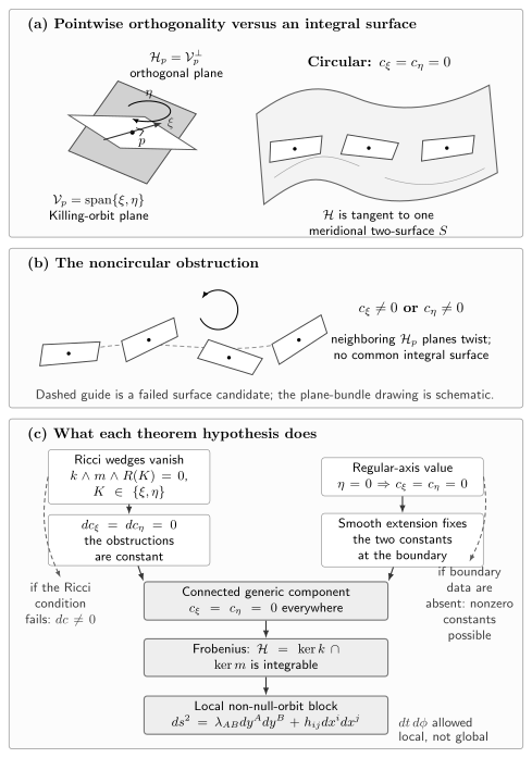
On the generic region where $\mathcal V=\operatorname{span}\{\xi,\eta\}$ is nondegenerate, $\mathcal H=\mathcal V^\perp$ is a rank-two distribution. Circularity means that $\mathcal H$ integrates to meridional two-surfaces, equivalently $c_\xi=c_\eta=0$. The Ricci circularity conditions make these obstruction scalars constant; a regular axis fixes their values to zero, and connectedness propagates the result before Frobenius gives the local block form. Without the Ricci conditions or a boundary value, orthogonal transitivity need not follow. The plane drawing and proof layout are schematic, not a coordinate embedding or a global-topology claim; a $dt\,d\phi$ term remains allowed.

Why the theorem works

Define the full twist one-form of a Killing field $K$ and the two circularity scalars by

$$\tau(K)=*\!\left(K^\flat\wedge dK^\flat\right), \qquad c_\xi=\iota_\eta\tau(\xi), \qquad c_\eta=-\iota_\xi\tau(\eta).$$

The contraction identities give exactly

$$c_\xi=*\!\left(k\wedge m\wedge dk\right), \qquad c_\eta=*\!\left(k\wedge m\wedge dm\right).$$

So Frobenius is equivalent to $c_\xi=c_\eta=0$. With the site’s curvature convention, signature $(-,+,+,+)$, and positive orientation, a Killing field obeys

$$d\tau(K)=2*\!\left(K^\flat\wedge R(K)\right).$$

The factor $2$ is important: some references define the twist as $\tfrac12\tau$. Because $[\xi,\eta]=0$ and both fields are Killing,

$$\mathcal L_\eta\tau(\xi)=0, \qquad \mathcal L_\xi\tau(\eta)=0.$$

Cartan’s identity $\mathcal L_X=d\iota_X+\iota_Xd$ then gives, with no unresolved sign choice,

$$dc_\xi=2*\!\left(k\wedge m\wedge R(\xi)\right), \qquad dc_\eta=2*\!\left(k\wedge m\wedge R(\eta)\right).$$

This is the engine of the theorem. The Ricci conditions make $c_\xi$ and $c_\eta$ constant on $\mathcal U_*$. Smooth extension to the regular axis gives

$$\left.c_\xi\right|_{\mathcal A} =\left.c_\eta\right|_{\mathcal A}=0,$$

because every defining four-form contains $m=\eta^\flat=0$ there. The constants on $\mathcal U_*$ therefore vanish. Frobenius supplies the local meridional surfaces, and the commuting Killing flows carry meridional coordinates from one such surface to neighboring orbits. This proof, including the half-twist normalization used there, is displayed in Heusler 1995, §2, printed pp. 3–4, Eqs. (7)–(11), Open PDF and reviewed in Chruściel, Costa, and Heusler 2012, §8.1, printed pp. 42–43, Eqs. (8.1)–(8.5), Open PDF.

The hypotheses have different jobs:

Hypothesis	What it contributes
$[\xi,\eta]=0$ and both fields Killing	Makes the twist forms invariant along the other symmetry flow.
Ricci circularity	Gives $dc_\xi=dc_\eta=0$, hence constancy—not yet zero.
Regular-axis or equivalent boundary data	Fixes both constants to zero.
Connected component	Propagates that zero value throughout the component.
$\det\lambda\ne0$	Makes orbit and orthogonal planes complementary, allowing a nonsingular local $2+2$ block.
Additional topology and boundary control	Needed only for global orbit-space or Weyl coordinates; Frobenius does not provide these.

What the matter conditions mean

Einstein’s equation with cosmological constant gives, for either $K=\xi$ or $K=\eta$,

$$R(K)=8\pi G\!\left[T(K)-\frac12T K^\flat\right]+\Lambda K^\flat.$$

Wedge with $k\wedge m$. The trace and cosmological terms contain a repeated $k$ or $m$, so

$$k\wedge m\wedge R(K) =8\pi G\,k\wedge m\wedge T(K).$$

On a nondegenerate orbit patch, the right-hand side vanishes precisely when $T(K)$ lies in the span of $k$ and $m$. In adapted language, the stress tensor has no orbit–meridional components $T_{Ai}$. This is the invariant content of “no meridional momentum flux” in the circularity theorem.

Matter model	Does circularity follow from the stated symmetry?
Vacuum, with or without $\Lambda$	Yes. $R(K)$ is proportional to $K^\flat$, so the wedge contains a repeated one-form.
Source-free Maxwell field	Yes, if $dF=d{*F}=0$, $\mathcal L_\xi F=\mathcal L_\eta F=0$, and $F$ extends smoothly to the axis. Then $F(\xi,\eta)$ and $({*F})(\xi,\eta)$ are constant and the axis sets both to zero; the Maxwell stress has no orbit–meridional block.
Symmetry-invariant minimally coupled scalar map	Yes. If $\mathcal L_\xi\Phi=\mathcal L_\eta\Phi=0$, then $T(K)$ is proportional to $K^\flat$ for either Killing field.
Perfect fluid with circular flow	Yes when $u$ lies in $\operatorname{span}\{\xi,\eta\}$; a meridional component of $u$ can spoil the condition.
Non-Abelian Yang–Mills field	Not in general. Gauge-covariant field equations and symmetry inheritance alone do not force the two contractions that vanish in Maxwell theory.

For Maxwell theory, “symmetry inheritance” here means invariance of $F$ itself, not merely invariance of its stress tensor; fields that inherit a symmetry only up to a duality rotation require separate analysis. The Abelian and non-Abelian distinction is worked out in Chinea and Navarro-Lérida 2002, printed pp. 1–2, Eqs. (1), (2), and (12)–(16), Open PDF.

Two hypotheses, two counterexamples

The following examples isolate the two logical inputs instead of dropping several hypotheses at once.

Ricci circularity without an axis value

Take $q\ne0$, make $\phi$ periodic, and consider

$$ds^2=-(dt+qx\,dy)^2+d\phi^2+dx^2+dy^2, \qquad \xi=\partial_t, \qquad \eta=\partial_\phi.$$

The fields commute, but the $U(1)$ action is free: $g(\eta,\eta)=1$, so there is no fixed axis. With orientation $dt\wedge d\phi\wedge dx\wedge dy>0$,

$$k=-(dt+qx\,dy), \qquad m=d\phi, \qquad dk=-q\,dx\wedge dy,$$

and therefore

$$k\wedge m\wedge dk =q\,dt\wedge d\phi\wedge dx\wedge dy, \qquad c_\xi=-q.$$

The exact Ricci wedges vanish, so $dc_\xi=dc_\eta=0$ exactly as the theorem predicts. But the nonzero constant has no axis value to force it to zero. This is a cyclic, axis-free geometry—not an axisymmetric one under the definition requiring a fixed set—and it is not circular.

A regular axis with a Ricci source

Now let $\phi$ have period $2\pi$ and set

$$ds^2=-(dt+\alpha R^2dz)^2+dR^2+R^2d\phi^2+dz^2, \qquad \alpha\ne0.$$

The axis $R=0$ is smooth: in Cartesian coordinates, $R^2=x^2+y^2$, and the $(R,\phi)$ sector has the ordinary flat-axis form. For $\xi=\partial_t$, $\eta=\partial_\phi$, and orientation $dt\wedge dR\wedge d\phi\wedge dz>0$,

$$k\wedge m\wedge dk =-2\alpha R^3\,dt\wedge dR\wedge d\phi\wedge dz, \qquad c_\xi=2\alpha R^2.$$

Thus $c_\xi$ does vanish at the axis, but $dc_\xi=4\alpha R\,dR$ away from it. The Ricci circularity condition is necessarily nonzero there and sources the obstruction. Axis data alone are not enough.

Coordinates can hide or create cross terms

Circularity says that a block chart exists locally; it does not say that every symmetry-adapted chart already has that form. Start with cylindrical Minkowski spacetime and put $\tau=t+f(R)$. Then

$$ds^2=-d\tau^2+2f'(R)\,d\tau\,dR +\left[1-f'(R)^2\right]dR^2+R^2d\phi^2+dz^2.$$

The displayed $d\tau\,dR$ term mixes an orbit and a meridional coordinate, but $\xi=\partial_\tau$ has dual

$$\xi^\flat=-d\tau+f'(R)dR=-dt,$$

so $d\xi^\flat=0$ and both circularity scalars vanish. Returning to $t$ removes the cross term. Conversely, rotating cylindrical coordinates produce a $dt\,d\phi$ term entirely within the Killing block; the geometry is still circular. The stationary and axial Killing geometry page explains why neither cross term alone is an invariant rotation test.

Frobenius supplies local leaves and local block coordinates on non-null orbit patches. It does not supply a global product, global Weyl–Papapetrou coordinates, half-plane orbit-space topology, regular extension across an axis or horizon, an event-horizon interpretation, or global twist and Ernst potentials. Those require additional field equations, topology, boundary data, and regularity. The later discussion of ergoregions, Killing horizons, and axis structure keeps these degenerations separate.

Common pitfalls

Circular is not static. Circularity concerns a rank-two distribution orthogonal to two symmetry fields. Staticity concerns hypersurface orthogonality of a timelike Killing field. Kerr’s domain of outer communications is circular but not static when its angular momentum is nonzero.

Commuting does not mean integrable orthogonal planes. Commutation integrates the orbit distribution $\mathcal V$; it does not integrate the different distribution $\mathcal H=\mathcal V^\perp$. The Ricci and boundary steps bridge that gap.

A periodic coordinate is not automatically an axial symmetry. A genuine axial action has a fixed set. The first counterexample has closed free $U(1)$ orbits but no axis, so it deliberately lacks the boundary datum used by the theorem.

A local block is not a global Weyl chart. The determinant condition and Frobenius theorem are local. Global quotient topology, axes, horizons, and harmonic orbit-space coordinates remain separate questions.

Exercises

1. Recover the codimension-two Frobenius test

Let $\mathcal H=\ker k\cap\ker m$, with $k$ and $m$ independent. Show that $\mathcal H$ is integrable if and only if

$$k\wedge m\wedge dk=0, \qquad k\wedge m\wedge dm=0.$$

Solution

For vector fields $X,Y\in\mathcal H$, one has $k(X)=k(Y)=0$. The exterior-derivative identity gives

$$dk(X,Y)=X[k(Y)]-Y[k(X)]-k([X,Y])=-k([X,Y]),$$

and similarly $dm(X,Y)=-m([X,Y])$. Hence $[X,Y]\in\mathcal H$ exactly when both two-forms vanish on pairs of vectors in $\mathcal H$. Because $k,m$ are independent, a two-form vanishes on $\mathcal H\times\mathcal H$ exactly when wedging it with $k\wedge m$ gives zero. This yields the two displayed conditions.

2. Translate Ricci circularity into matter flux

Use Einstein’s equation to derive the stress-energy wedge conditions. Verify them in vacuum with $\Lambda$ and interpret them in a block-adapted basis.

Solution

For $K=\xi$ or $\eta$,

$$R(K)=8\pi G\!\left[T(K)-\frac12TK^\flat\right]+\Lambda K^\flat.$$

The trace and cosmological terms vanish after wedging with $k\wedge m$, because $K^\flat$ is one of those two factors. Thus Ricci circularity is equivalent to

$$k\wedge m\wedge T(\xi)=0, \qquad k\wedge m\wedge T(\eta)=0.$$

In vacuum $T=0$, so these hold immediately, with or without $\Lambda$. In a coframe split into orbit and meridional directions, the equations say $T(\xi)$ and $T(\eta)$ have no meridional components, equivalently $T_{Ai}=0$. The theorem still needs a boundary value: the field equations make $c_\xi,c_\eta$ constant, while the regular axis makes those constants zero.

3. Diagnose the regular-axis counterexample

For

$$ds^2=-(dt+\alpha R^2dz)^2+dR^2+R^2d\phi^2+dz^2,$$

compute $k\wedge m\wedge dk$ and $c_\xi$. Which theorem hypothesis fails?

Solution

Here

$$k=-(dt+\alpha R^2dz), \qquad m=R^2d\phi, \qquad dk=-2\alpha R\,dR\wedge dz.$$

Therefore

$$k\wedge m\wedge dk =-2\alpha R^3\,dt\wedge dR\wedge d\phi\wedge dz.$$

Since $\sqrt{-g}=R$ and $*\operatorname{vol}=-1$ for signature $(-,+,+,+)$, $c_\xi=2\alpha R^2$. It vanishes at $R=0$ but is nonzero for $R>0$, with $dc_\xi=4\alpha R\,dR$. The axis and connectedness hypotheses hold; the Ricci circularity condition fails and supplies this derivative through the twist identity.

4. Diagnose the missing boundary value

For the axis-free metric with $A(x)=qx$, verify $c_\xi=-q$ and explain why Ricci circularity still does not imply orthogonal transitivity. Then list two global conclusions that the circularity theorem would not prove even if $c_\xi=c_\eta=0$.

Solution

The calculation above gives

$$k\wedge m\wedge dk=q\,dt\wedge d\phi\wedge dx\wedge dy.$$

The determinant is $-1$, so the displayed coordinate volume is the metric volume; in Lorentzian signature its Hodge dual is $-1$. Hence $c_\xi=-q$, while $c_\eta=0$. Both are constant and the exact Ricci wedges vanish, but no fixed axis or other boundary condition sets the nonzero constant to zero. Thus Ricci circularity gives constancy without circularity. Even when both scalars vanish, the theorem alone gives neither global Weyl coordinates nor a global product topology; it also does not identify a degenerating boundary as an event horizon.

References

• Carter, Brandon. “Killing Horizons and Orthogonally Transitive Groups in Space-Time.” Journal of Mathematical Physics 10 (1969): 70–81. DOI: 10.1063/1.1664763.
• Chinea, Francisco J., and Francisco Navarro-Lérida. “Stationary Axisymmetric SU(2) Einstein–Yang–Mills Fields with Restricted Circularity Conditions Are Abelian.” Physical Review D 65 (2002): 064010. DOI: 10.1103/PhysRevD.65.064010; Open PDF.
• Chruściel, Piotr T., João Lopes Costa, and Markus Heusler. “Stationary Black Holes: Uniqueness and Beyond.” Living Reviews in Relativity 15 (2012): 7. DOI: 10.12942/lrr-2012-7; Open PDF.
• Heusler, Markus. “The Uniqueness Theorem for Rotating Black Hole Solutions of Self-Gravitating Harmonic Mappings.” Classical and Quantum Gravity 12 (1995): 2021–2036. DOI: 10.1088/0264-9381/12/8/017; Open PDF.
• Wald, Robert M. General Relativity. Chicago: University of Chicago Press, 1984. Publisher record.