Multipole Expansion and Radiation Zones

Guiding question: Why do conservation laws suppress the lowest radiative multipoles for many sources?

A conserved total charge cannot oscillate, so its monopole field cannot carry time-dependent radiation. In electromagnetism the leading radiation from a localized nonrelativistic source is therefore usually electric dipole radiation. Analogous conservation laws can remove further low multipoles in other theories, but the conclusion must be derived from that theory’s source and conservation equations.

Required background. Ordinary Differential Equations provides initial-value problems, linearization, and asymptotic solution methods; Classical Field Theory provides field actions, Euler–Lagrange equations, and gauge redundancy. Helpful background. Calculus and Linear Algebra provides multivariable differentiation, linear maps, inner products, and basis changes; Partial Differential Equations and Green Functions provides characteristics, boundary data, distributions, and Green-function methods.

Electromagnetic dipole radiation

Use $c=1$, rationalized Heaviside-Lorentz units, and retarded time $u=t-r$. For a compact source of size $d$, the retarded solution of a scalar wave equation is

$$\psi(t,\mathbf x) =\frac{1}{4\pi}\int d^3x'\, \frac{s(t-|\mathbf x-\mathbf x'|,\mathbf x')} {|\mathbf x-\mathbf x'|}.$$

At $r\gg d$, with $\mathbf n=\mathbf x/r$,

$$|\mathbf x-\mathbf x'| =r-\mathbf n\mathbin{\cdot}\mathbf x'+O(d^2/r), \qquad \frac1{|\mathbf x-\mathbf x'|}=\frac1r+O(d/r^2).$$

Taylor expanding the retarded source gives

$$\psi =\frac{1}{4\pi r} \left[ Q(u)+n_i\dot D_i(u) +\frac12n_in_j\ddot Q_{ij}(u)+\cdots \right]+O(r^{-2}),$$

where

$$Q=\int s\,d^3x',\quad D_i=\int x'_i s\,d^3x',\quad Q_{ij}=\int x'_ix'_j s\,d^3x'.$$

For a component varying as $e^{-i\omega t}$, set $k=\omega$ in units with $c=1$. The physical wavelength is $\lambda_{\rm phys}=2\pi/k$, while the multipole expansion is controlled by

$$\boxed{kd\ll1.}$$

Each additional moment supplies one power of $d$ and one additional time derivative supplies one power of $k$, so successive radiative amplitudes are typically suppressed by $kd$. A scalar source with nonconserved $Q$ may radiate monopole waves; conservation is doing physical work, not merely organizing notation.

For electromagnetism, charge conservation gives

$$\dot Q=0,\qquad \int\mathbf J\,d^3x=\dot{\mathbf p}, \qquad \mathbf p=\int\rho\,\mathbf x\,d^3x.$$

The first identity removes electric monopole radiation. The second follows by integrating $\partial_t\rho+\boldsymbol\nabla\mathbin{\cdot}\mathbf J=0$ against $\mathbf x$ and discarding surface current at infinity.

Expanding the retarded potentials then yields the leading $1/r$ fields

$$\boxed{ \mathbf E_{\rm rad} =\frac{\mathbf n\times(\mathbf n\times\ddot{\mathbf p}(u))} {4\pi r}, \qquad \mathbf B_{\rm rad}=\mathbf n\times\mathbf E_{\rm rad}. }$$

They are transverse and in phase. The angular power is

$$\frac{dP}{d\Omega} =\frac{|\mathbf n\times\ddot{\mathbf p}|^2}{16\pi^2},$$

and integration gives the instantaneous power $P=|\ddot{\mathbf p}|^2/(6\pi)$.

The next two moments are the magnetic dipole and trace-free electric quadrupole,

$$\mathbf m=\frac12\int \mathbf x\times\mathbf J\,d^3x, \qquad Q^{\rm E}_{ij}=\int \rho \left(3x_ix_j-|\mathbf x|^2\delta_{ij}\right)d^3x.$$

For a nonrelativistic source with characteristic speed $v_{\rm src}\sim kd\ll1$, dimensional estimates give

$$|\mathbf m|\sim kd\,|\mathbf p|, \qquad k|Q^{\rm E}|\sim kd\,|\mathbf p|.$$

Magnetic-dipole and electric-quadrupole radiation are therefore generally one order $kd$ below electric-dipole radiation in field amplitude. If symmetry or dynamics makes $\mathbf p$ vanish, either correction can instead be the leading channel. Tong derives the electric-dipole field and power and then both corrections in Tong 2015, §§6.2.1–6.2.4, pp. 144–152 (official PDF).

Source and exterior radial regimes

For a source dominated by angular frequency $\omega=k$:

• The source or interior region, $r\lesssim d$, depends on the source’s internal structure. Exterior multipole falloffs do not apply there.
• The exterior near zone, $d\ll r$ and $kr\ll1$, is dominated by quasistatic fields such as exterior $r^{-3}$ dipole terms.
• The induction zone, $d\ll r$ and $kr\sim1$, mixes $r^{-3}$, $r^{-2}$, and $r^{-1}$ behavior.
• The radiation zone, $r\gg d$ and $kr\gg1$, is dominated by transverse $r^{-1}$ fields with finite flux through large spheres, comparing radii at fixed retarded time $u=t-r$.

The ordered hierarchy, including a parametrically separated exterior near zone, requires $kd\ll1$; this is the same source condition that controls the long-wavelength multipole expansion. Merely taking $r$ large does not make an electrically large source a point dipole. Conversely, an exterior near-zone field can vary in time without representing freely escaping radiation. These regimes are asymptotic overlaps, not sharp circles at a universal numerical value of $kr$.

The figure separates the source or interior from all three exterior regimes. Read outward from $r\lesssim d$ through $d\ll r$ with $kr\ll1$, then $kr\sim1$, and finally $r\gg d$ with $kr\gg1$. The separate note records the independent source condition $kd\ll1$, and the drawn circles are not sharp physical boundaries.

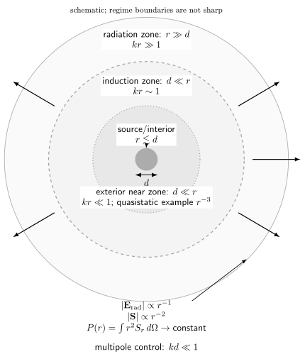
A compact source has a controlled multipole hierarchy only when $kd\ll1$. Outside it, $kr$ separates the exterior near, induction, and radiation regimes: $kr\ll1$, $kr\sim1$, and $kr\gg1$, with $d\ll r$ for the exterior expansion and $r\gg d$ in the far-zone claim. The circles are schematic, not sharp boundaries. The radial falloffs and $P(r)$ limit hold at fixed retarded time $u=t-r$; the power limit also applies after cycle averaging a periodic source.

Flux and the meaning of radiation

The $1/r$ falloff is singled out in three spatial dimensions because a quadratic energy flux then scales as $1/r^2$. To compare the same stage of emission at different radii, hold $u=t-r$ fixed. The luminosity through a sphere is then

$$P(u,r)=\int r^2\,\mathbf S(u+r,r\mathbf n)\mathbin{\cdot}\mathbf n\,d\Omega.$$

As $r\to\infty$ at fixed $u$, this approaches a finite limiting luminosity $P_\infty(u)$ even when the angular pattern is anisotropic. It may vary with retarded time; spheres compared at the same coordinate time generally sample different stages of emission. For periodic sources one can instead compare cycle-averaged power. Faster-falling terms store or exchange energy locally but contribute no finite flux in this large-radius limit. This scaling is a diagnostic, not a complete definition: one must also impose retarded boundary conditions and identify the stress-energy or conserved current whose outward flux is being measured.

The lowest allowed multipole is theory dependent. Electromagnetic charge conservation removes a time-dependent electric monopole, but leaves an electric dipole. For an isolated Newtonian mass distribution, mass conservation fixes the mass monopole and momentum conservation makes the mass dipole’s second derivative vanish; in the center-of-mass frame the dipole itself can be set to zero. These are the conservation-law ingredients behind leading quadrupole radiation in weak-field, slow-motion general relativity. Establishing the gravitational radiation law, its normalization, and its gauge-invariant meaning requires the gravitational field equations and is developed in the gravitational-radiation volume; the scalar-wave calculation here does not derive it.

Transfer task: an oscillating dipole

Let $\mathbf p(t)=p_0\cos(\omega t)\widehat{\mathbf z}$. Find the radiation pattern and cycle-averaged total power.

Solution

Since $|\mathbf n\times\widehat{\mathbf z}|=\sin\theta$,

$$\frac{dP}{d\Omega} =\frac{p_0^2\omega^4}{16\pi^2} \cos^2[\omega(t-r)]\sin^2\theta.$$

The radiation vanishes on the dipole axis and is maximal in the equatorial plane. Averaging $\cos^2$ over a cycle and integrating $\int\sin^2\theta\,d\Omega=8\pi/3$ gives

$$\boxed{\langle P\rangle =\frac{p_0^2\omega^4}{12\pi}.}$$

The $\omega^4$ scaling is a strong low-frequency suppression; the approximation also requires the source compactness condition $kd=\omega d\ll1$.

Continue to Scattering, Resonance, and Linear Response to see how an external wave probes a system and excites its damped modes.

References

• David Tong, Lectures on Electromagnetism, University of Cambridge, 2015, §§6.1–6.2.4, pp. 134–152 (official PDF).