Retarded and Advanced Green Functions

Guiding question: Which physical choice distinguishes the retarded solution from other solutions of the same field equation?

The differential operator does not choose an arrow of response. The retarded Green function is selected by a support condition: its response lies in the causal future of the source event. The advanced Green function instead has past support. Initial data, incoming-radiation conditions, and experimental preparation determine which inverse is physical.

Required background. Ordinary Differential Equations provides initial-value problems, linearization, and asymptotic solution methods; Classical Field Theory provides field actions, Euler–Lagrange equations, and gauge redundancy; Partial Differential Equations and Green Functions provides characteristics, boundary data, distributions, and Green-function methods. Helpful background. Calculus and Linear Algebra provides multivariable differentiation, linear maps, inner products, and basis changes.

Source response

Let

$$L=\partial_t^2-\nabla^2=-\Box$$

in $3+1$ dimensional Minkowski spacetime, with $c=1$ and signature $(-,+,+,+)$. A fundamental solution satisfies

$$L G(t,\mathbf x)=\delta(t)\delta^{(3)}(\mathbf x).$$

The retarded and advanced choices are

$$\boxed{ G_{\rm ret}(t,\mathbf x) =\frac{\delta(t-r)}{4\pi r},\qquad G_{\rm adv}(t,\mathbf x) =\frac{\delta(t+r)}{4\pi r}, } \qquad r=|\mathbf x|.$$

Their supports lie respectively on the future and past null cones. They differ by a homogeneous solution because $L(G_{\rm ret}-G_{\rm adv})=0$. MIT 18.155 constructs the forward fundamental solution and proves its support property in Jaffe 2016, Lecture 21, §§0–6, pp. 1–6 (official PDF).

The normalization can be checked without manipulating $1/r$ at the origin. After a spatial Fourier transform, the retarded mode is

$$g_k(t)=\theta(t)\frac{\sin(kt)}{k}, \qquad k=|\mathbf k|.$$

Away from $t=0$ it solves $(\partial_t^2+k^2)g_k=0$. Across $t=0$ its derivative jumps by one,

$$g_k'(0^+)-g_k'(0^-)=1,$$

so distributionally $(\partial_t^2+k^2)g_k=\delta(t)$. Inverting the spatial transform gives $G_{\rm ret}=\delta(t-r)/(4\pi r)$ with future support and the required unit delta source.

For $L\psi=s$ and vanishing incoming homogeneous data, convolution gives

$$\psi_{\rm ret}(t,\mathbf x) =\int d^3x'\, \frac{s(t-|\mathbf x-\mathbf x'|,\mathbf x')} {4\pi|\mathbf x-\mathbf x'|}.$$

Only the source at retarded time contributes. Directly applying $L$ under the convolution yields $s$, while the support of $G_{\rm ret}$ guarantees that a source cannot influence earlier events.

The same support choice appears as a pole prescription. With the transform pair normalized by

$$G(t,\mathbf x) =\int\frac{d\omega}{2\pi} \frac{d^3k}{(2\pi)^3} e^{i(\mathbf k\cdot\mathbf x-\omega t)} \widetilde G(\omega,\mathbf k),$$

the two inverses are boundary values

$$\widetilde G_{\rm ret} =\frac{1}{|\mathbf k|^2-(\omega+i0)^2}, \qquad \widetilde G_{\rm adv} =\frac{1}{|\mathbf k|^2-(\omega-i0)^2}.$$

Here $i0$ means the limit from positive imaginary displacement. Both retarded poles lie below the real $\omega$ axis. For $t\lt0$, closing the contour in the upper half-plane encloses no pole, so the response vanishes; the advanced prescription reverses this support. This contour check fixes the sign for the site’s $e^{-i\omega t}$ convention.

This is not the most general solution:

$$\psi=\psi_{\rm hom}+G_{\rm ret}*s.$$

The homogeneous term carries freely specified Cauchy data or incoming waves. Replacing $G_{\rm ret}$ by $G_{\rm adv}$ and changing $\psi_{\rm hom}$ can represent the same local source equation with different global preparation. Tong uses the opposite operator, $(\nabla^2-\partial_t^2)G=\delta$, and therefore writes the retarded kernel with an overall minus sign. Multiplying that Green-function equation by $-1$ gives the convention used here; compare Tong 2015, §§6.1.1–6.1.2, pp. 135–142 (official PDF).

Boundary condition, not algebraic inevitability

In a laboratory, a source is switched on after initial data are prepared and detectors register later signals; the retarded solution matches that intervention. The advanced solution is mathematically legitimate but would encode incoming radiation coordinated to converge before or onto the source. Time-symmetric choices such as $(G_{\rm ret}+G_{\rm adv})/2$ solve the same local equation and appear in specialized formulations, but they impose different global data.

The simple cone-only formula is dimension- and operator-dependent. In $3+1$ dimensions the massless flat Green function has sharp null-cone support. Massive fields, other spatial dimensions, media, boundaries, or curved spacetimes can have support inside the cone. Retarded does not mean “only on the cone”; it means no support outside the causal future.

The figure shows the general causal-support statement rather than the special sharp-cone case. In this reused schematic, its labels $P$ and $f$ denote this page’s $L$ and $s$, respectively. The compact diamond $K=\operatorname{supp}s$ has exact causal future and past boundaries: for a diamond $|t|+|x|\leq a$, these are $t=|x|-a$ and $t=a-|x|$. The dashed lines mark those boundaries, and the shading marks allowed support, not field amplitude or a guarantee of a nonzero signal throughout either region. These dashed envelopes are specific to the stated diamond; for an extended source blob they are not meant as the exact boundary of $J^\pm(\operatorname{supp}s)$ without the same shape assumption. A different source support requires its own causal envelope.

The massless 3+1-dimensional flat Green function discussed here has support only on the null cone. Its convolution with a source extended in time can nevertheless fill a region, because different observation events receive null-cone contributions from different source events. With the retarded-minus-advanced orientation,

$$E=G_{\rm ret}-G_{\rm adv}, \qquad L(Es)=s-s=0.$$

Thus the causal propagator produces a homogeneous solution everywhere in the distributional sense, including within the source support: the two source terms cancel there as well.

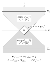
A compact source has retarded support only in its causal future and advanced support only in its causal past; with the declared convention, their difference is the causal propagator. Schematic and not to scale.

Common failures are to omit the homogeneous solution, treat “outgoing” and “retarded” as interchangeable in every time-dependent problem, or Fourier transform through poles without specifying a contour prescription. The familiar $i0$ rule is the frequency-domain encoding of a support choice.

Transfer task: a point source

Let $s(t,\mathbf x)=q(t)\delta^{(3)}(\mathbf x)$. Find the retarded field and check its static limit.

Solution

Substitution into the convolution gives

$$\boxed{\psi_{\rm ret}(t,r)=\frac{q(t-r)}{4\pi r}.}$$

No response occurs at radius $r$ before a source change has had time $r$ to arrive. If $q(t)=q_0$ is constant, then

$$\psi=\frac{q_0}{4\pi r},$$

the static Green function away from the origin. The advanced solution would contain $q(t+r)$ and respond to a future source value, displaying the physical distinction directly.

Continue to The Eikonal and Geometric-Optics Limits to approximate high-frequency homogeneous solutions by rays rather than source convolutions.

References

• Ethan Jaffe, MIT 18.155 Lecture 21: Forward Fundamental Solution to the Wave Equation, Massachusetts Institute of Technology, 2016, §§0–6, pp. 1–6 (official PDF).
• David Tong, Lectures on Electromagnetism, University of Cambridge, 2015, §§6.1.1–6.1.3, pp. 135–143 (official PDF).