Lapse, Shift, and Measurements in Noninertial Coordinates

A lapse gradient can produce position-dependent clock rates and acceleration-like terms; a shift can produce time–space cross terms and Coriolis-like effects; a curvilinear spatial metric can produce centrifugal-looking connection coefficients. All can occur in exactly flat spacetime. The decomposition organizes a coordinate choice, but measurements still require a specified observer four-velocity.

Required background. Special Relativity provides Minkowski causal geometry, four-vectors, and mass-shell kinematics; Relativistic Observers and Measurement provides observer rest spaces and invariant decompositions of measured quantities. Helpful background. Calculus and Linear Algebra provides multivariable differentiation, linear maps, inner products, and basis changes; Ordinary Differential Equations provides initial-value problems, linearization, and asymptotic solution methods.

Lapse, shift, and elapsed time

Write a metric foliated by surfaces of constant $t$ as

$$\boxed{ds^2=-N^2dt^2 +h_{ij}(dx^i+\beta^i dt)(dx^j+\beta^j dt).}$$

Here $N\gt0$ is the lapse, $\beta^i$ the shift, and $h_{ij}$ the positive spatial metric on a $t=\text{constant}$ slice. Expanding gives

$$g_{tt}=-N^2+\beta^2,\qquad g_{ti}=h_{ij}\beta^j,\qquad \beta^2=h_{ij}\beta^i\beta^j.$$

The future unit normal to the slices is

$$n=\frac{1}{N}\left(\partial_t-\beta^i\partial_i\right),$$

whereas the coordinate-grid worldlines have $x^i=\text{constant}$ and tangent $\partial_t=Nn+\beta$. These are generally different observer families, and a nonzero shift does not by itself imply spacetime curvature. In the figure, follow the normal advance between slices and then the tangential shift along the upper slice to see how their sum follows the coordinate-time line. The lapse, shift, and their coordinate meaning are derived in Gourgoulhon 2007, §§3.3.1–3.3.3, printed pp. 41–44, and §4.2.2, printed pp. 56–57.

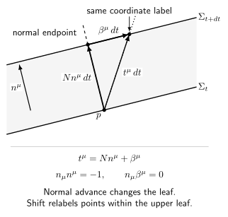
A coordinate-time displacement is the sum of normal proper advance N n dt and tangential coordinate shift beta dt. A coordinate line is normal only when the shift vanishes. Schematic and not to scale.

A fixed-coordinate curve is timelike only if

$$N^2\gt\beta^2.$$

Its proper time is

$$d\tau_{\rm grid}=\sqrt{N^2-\beta^2}\,dt.$$

Relative to the normal observer, its spatial velocity has slice components, squared speed, and Lorentz factor

$$v^i=\frac{\beta^i}{N},\qquad v^2=h_{ij}v^iv^j=\frac{\beta^2}{N^2}\lt1,\qquad \gamma_{\rm grid|n}=\frac{N}{\sqrt{N^2-\beta^2}}.$$

Thus $N$ alone is not the grid clock rate when the shift is nonzero: $d\tau_{\rm grid}=N\sqrt{1-v^2}\,dt$.

Measurements are projections, not coordinate components. An observer with unit four-velocity $w^\mu$ assigns a particle four-momentum $p^\mu$ the energy

$$E_{(w)}=-p_\mu w^\mu$$

and the spatial momentum

$$p_{\perp(w)}^\mu =\left(\delta^\mu{}_\nu+w^\mu w_\nu\right)p^\nu =p^\mu-E_{(w)}w^\mu.$$

The minus sign is fixed by $p^\mu=E_{(w)}w^\mu+p_{\perp(w)}^\mu$ and $w\mathbin{\cdot}p_{\perp(w)}=0$. The normal observer uses $w=n$; a normalized grid observer uses

$$w_{\rm grid} =\frac{\partial_t}{\sqrt{N^2-\beta^2}}.$$

They need not agree. Even when $p_t$ is conserved in a stationary chart, $-p_t$ is not automatically the locally measured energy.

Two flat-spacetime examples

For Rindler coordinates shifted so that the reference observer is at $\xi=0$,

$$ds^2=-(1+a\xi)^2dt^2+d\xi^2+dy^2+dz^2.$$

On the connected region $1+a\xi\gt0$, therefore, $N=1+a\xi$, $\beta^i=0$, and $h_{ij}=\delta_{ij}$. Normal and grid observers coincide. The normal congruence has spatial acceleration

$$a_i^{(n)}=D_i\ln N,$$

so $a_\xi^{(n)}=a/(1+a\xi)$. This follows directly from $n=N^{-1}\partial_t$: the only needed connection coefficient is $\Gamma^\xi{}_{tt}=Na$, and hence $(n\mathbin{\cdot}\nabla)n^\xi=a/N$. The general identity $a_i^{(n)}=D_i\ln N$ is derived in Gourgoulhon 2007, §3.3.3, printed pp. 43–44, Eqs. (3.16)–(3.18). The lapse gradient accounts for both the accelerometer profile and the redshift, even though every Riemann-tensor component is zero.

For uniformly rotating coordinates,

$$ds^2=-(1-\Omega^2r^2)dt^2 +2\Omega r^2dt\,d\phi+dr^2+r^2d\phi^2+dz^2.$$

One reads

$$N=1,\qquad \beta^\phi=\Omega,\qquad h_{ij}dx^idx^j=dr^2+r^2d\phi^2+dz^2.$$

The normal observers are inertial: $n=\partial_t-\Omega\partial_\phi$ is simply $\partial_T$ in the original inertial chart. The grid observers rotate and accelerate. Here $\beta^2=h_{\phi\phi}(\beta^\phi)^2=\Omega^2r^2$, so their admissibility condition is $N^2\gt\beta^2$, or $1\gt\Omega^2r^2$, reproducing the light cylinder. A shift is therefore not itself “motion of space”; it records how coordinate time lines thread successive spatial slices.

Which apparent gravitational effects are coordinate-made?

In a noninertial chart on Minkowski spacetime, a lapse gradient can mimic a uniform gravitational redshift and a support force. A shift and its spatial derivatives can generate Coriolis-like terms. Rotation of the grid produces centrifugal terms, and time-dependent rotation produces Euler-like terms. Curvilinear $h_{ij}$ contributes geometric connection terms even for inertial motion.

These appearances are useful, not fictitious in the sense of being unmeasurable: a supported accelerometer really reads nonzero, and a rotating interferometer really measures a Sagnac delay. What is coordinate-dependent is their description as forces or metric components. A curvature calculation supplies the decisive check. For all examples in this chapter, $R^\rho{}_{\sigma\mu\nu}=0$ wherever the coordinates are regular.

Common errors are to infer curvature from nonzero Christoffel symbols, to call every $g_{tt}=0$ surface an event horizon, or to discuss “the observer” without saying whether it is normal to the slices or fixed on the coordinate grid. Gourgoulhon 2007, §4.2.4, printed p. 59 explains how lapse and shift propagate the slicing and spatial coordinates.

Transfer task: a pure constant shift

In inertial coordinates set $t=T$ and $x=X-VT$, where $|V|\lt1$. Decompose the metric and identify both observer families.

Solution

Since $dX=dx+Vdt$,

$$ds^2=-dt^2+(dx+Vdt)^2+dy^2+dz^2.$$

Thus $N=1$, $\beta^x=V$, and $h_{ij}=\delta_{ij}$. The normal is

$$n=\partial_t-V\partial_x=\partial_T,$$

so normal observers are at rest in the original inertial chart. Grid observers have $x=\text{constant}$, hence $X=VT+\text{constant}$; they move inertially at speed $V$ and accumulate $d\tau_{\rm grid}=\sqrt{1-V^2}\,dt$. All metric components are constant, so the Christoffel symbols and curvature vanish. A nonzero shift need imply neither rotation nor force.

Continue to Classical Fields and Electromagnetism, where the same observer projections separate electric and magnetic fields while Lorentz invariants remain frame-independent.

References

• Éric Gourgoulhon, “3+1 Formalism and Bases of Numerical Relativity”, §§3.3.1–3.3.3, printed pp. 41–44; §4.2.2, printed pp. 56–57; and §4.2.4, printed p. 59, arXiv:gr-qc/0703035v1, 2007.

Further reading

• Éric Gourgoulhon, Special Relativity in General Frames: From Particles to Astrophysics, Chapters 12–13, Graduate Texts in Physics, Springer, 2013; consult the author’s errata.