Uniform Acceleration and Rindler Wedges

An observer accelerating eternally along one fixed spatial direction, with constant nonzero proper acceleration, follows a hyperbola that approaches two null lines. With null coordinates $U=T-X$ and $V=T+X$, the complete right-accelerated orbit can receive signals only from $U\lt0$ and can send signals only into $V\gt0$. Their intersection, $U\lt0\lt V$, is the right Rindler wedge: the region of two-way communication on which the stationary Rindler chart lives. The orbit’s causal past and causal future separately extend beyond that wedge. Its horizons are observer-dependent causal boundaries, not curvature singularities or a global black-hole event horizon.

Required background. Special Relativity provides Minkowski causal geometry, four-vectors, and mass-shell kinematics; Relativistic Observers and Measurement provides observer rest spaces and invariant decompositions of measured quantities. Helpful background. Calculus and Linear Algebra provides multivariable differentiation, linear maps, inner products, and basis changes; Ordinary Differential Equations provides initial-value problems, linearization, and asymptotic solution methods.

From one orbit to a Rindler congruence

For motion along $X$, introduce rapidity $\vartheta$:

$$u^\mu=(\cosh\vartheta,\sinh\vartheta,0,0).$$

Then

$$a^\mu=\frac{d\vartheta}{d\tau}(\sinh\vartheta,\cosh\vartheta,0,0), \qquad \alpha=\left|\frac{d\vartheta}{d\tau}\right|.$$

For signed constant acceleration $a\gt0$, choose the inertial origin at the center of the hyperbola and let the observer be instantaneously at rest at $(T,X)=(0,a^{-1})$. Then $\vartheta=a\tau$ and

$$\boxed{T(\tau)=a^{-1}\sinh(a\tau), \qquad X(\tau)=a^{-1}\cosh(a\tau).}$$

Consequently $X^2-T^2=a^{-2}$ and $dX/dT=\tanh(a\tau)$. The worldline approaches $X=|T|$ but never reaches either null line at finite proper time. The same hyperbolic solution is derived with explicit factors of $c$ in Hughes 2024, Lecture 14, §14.1, printed pp. 110–111, Eqs. (14.1)–(14.5).

Introduce coordinates $(\eta,\rho,y,z)$ by

$$T=\rho\sinh(a\eta), \qquad X=\rho\cosh(a\eta), \qquad \rho\gt0.$$

This is the traditional extended-tetrad construction in Pauri and Vallisneri 2000, §4, printed pp. 6–7, Eqs. (10)–(12). Direct substitution gives

$$\boxed{ds^2=-(a\rho)^2d\eta^2+d\rho^2+dy^2+dz^2.}$$

Every fixed-$\rho$ curve is uniformly accelerated, but its proper acceleration is $1/\rho$, not the same constant for the entire congruence. Indeed, its proper time is $d\sigma=a\rho\,d\eta$, so its normalized tangent and four-acceleration are

$$u^\mu=(\cosh a\eta,\sinh a\eta,0,0), \qquad A^\mu=\frac1\rho(\sinh a\eta,\cosh a\eta,0,0).$$

Thus $u^2=-1$, $u\mathbin{\cdot}A=0$, and $A^2=\rho^{-2}$. The original observer is at $\rho=1/a$, where $\eta$ equals its proper time. This spatial variation is exactly what permits the coordinate distances between neighboring observers to remain constant.

The null-coordinate form of the map is especially useful:

$$U=-\rho e^{-a\eta}, \qquad V=\rho e^{a\eta}.$$

It makes $U\lt0\lt V$ immediate. Equivalently, the inverse relations are

$$\rho=\sqrt{X^2-T^2}, \qquad \tanh(a\eta)=\frac{T}{X}.$$

They exist only when $X\gt|T|$, the right Rindler wedge. At finite $\eta$, the limit $\rho\to0$ maps only to the origin $U=V=0$. A generic point on the future horizon $U=0$, $V\gt0$ instead requires the correlated limit $\rho\to0$, $\eta\to+\infty$ with $\rho e^{a\eta}$ fixed; a generic point on the past horizon $V=0$, $U\lt0$ requires $\eta\to-\infty$ with $\rho e^{-a\eta}$ fixed. The Rindler metric degenerates in these limiting coordinates, but the inertial metric remains regular.

The null surfaces $X=\pm T$ are horizons for the chosen uniformly accelerated worldlines: causal curves from parts of Minkowski spacetime cannot cross them in the required direction and still meet those worldlines. Yet inertial observers cross them uneventfully. Calling them acceleration or Rindler horizons preserves the distinction from the observer-independent event horizon assigned to an entire asymptotic spacetime in black-hole geometry. The chart, its flat metric, and this causal restriction are exhibited in Hughes 2024, Lecture 14, §14.5, printed pp. 117–119, Eqs. (14.37)–(14.45).

The four-wedge picture makes the restricted chart visible. Its boost generator is

$$\chi=\partial_\eta =a\left(X\partial_T+T\partial_X\right).$$

Its time component is $\chi^T=aX$, so it is future-directed in the right wedge and past-directed in the left. Inspect the null boundaries and the hyperbolic orbits: a fixed-$\rho$ observer remains in one lateral wedge, while the same global boost generator has opposite time orientation on the mirror orbit in the other lateral wedge.

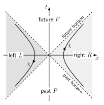
Null lines divide Minkowski space into four wedges; constant-acceleration hyperbolae approach the horizons. Arrows show the same boost generator futureward on the right and pastward on the left. Horizon names refer to the right-wedge observer; schematic, not to scale.

Accelerated-clock redshift

The Rindler lapse is $N=a\rho$. A fixed-$\rho$ clock accumulates

$$d\sigma=a\rho\,d\eta.$$

For a photon, stationarity conserves $\mathcal E=-p_\eta$. The local observer has $u=(a\rho)^{-1}\partial_\eta$, so the measured frequency is

$$\omega(\rho)=-p\mathbin{\cdot}u=\frac{\mathcal E}{a\rho}.$$

Thus two Rindler observers receiving the same null ray measure

$$\frac{\omega_2}{\omega_1}=\frac{\rho_1}{\rho_2}.$$

Light received at larger $\rho$ is redshifted. No spacetime curvature is needed; the sender and receiver belong to different accelerated worldlines. The clock-rate and spectral-shift calculation in the shifted coordinate $\rho=a^{-1}+x$ is worked through in Gourgoulhon 2010, PDF slides 28–30.

For a radial light signal, the null metric gives $d\rho/d\eta=\pm a\rho$. A signal sent outward from $\rho_1$ to $\rho_2\gt\rho_1$ takes coordinate time $\Delta\eta=a^{-1}\ln(\rho_2/\rho_1)$. Successive crests have the same coordinate separation at either end because the metric is stationary, but the local clock interval scales as $a\rho$. The larger interval at the receiver is the same redshift derived from the conserved photon energy.

Checks and common failures

• For the inertial limit, write $\rho=a^{-1}+\xi$ and recenter $X'=X-a^{-1}$. At fixed $(\eta,\xi)$, $a\to0$ gives $T\to\eta$, $X'\to\xi$, and the metric tends to inertial form.
• “Constant acceleration” must mean constant proper acceleration along one orbit. A Born-rigid Rindler family necessarily has $\alpha=1/\rho$.
• The Rindler construction also requires rectilinear acceleration. Uniform circular motion has constant proper-acceleration magnitude but does not follow these hyperbolae. A rocket that accelerates for a finite interval and then coasts forever has no future reception horizon of this type: an eventual timelike straight line can receive a signal from any fixed event in Minkowski spacetime if given enough time. Horizons depend on the complete history, not one accelerometer reading.
• The Rindler chart covers neither the future and past wedges nor the left wedge. This is a chart and congruence choice, not missing spacetime.
• A coordinate horizon can coincide with a causal horizon for specified observers without becoming a global event horizon or a curvature singularity.
• The classical Rindler horizon does not by itself establish Unruh radiation; that conclusion requires quantum field theory and a state choice.

Transfer task: a finite accelerating rocket

The rear of a rocket has proper acceleration $a_0$ and sits at $\rho_0=1/a_0$. Its front is a proper distance $L\gt0$ ahead on an $\eta=\text{constant}$ slice. Find the front acceleration and its clock rate relative to the rear.

Solution

The front is at $\rho_f=a_0^{-1}+L$, so

$$\boxed{a_f=\frac{1}{\rho_f}=\frac{a_0}{1+a_0L}}.$$

At equal $d\eta$, proper times obey

$$\frac{d\sigma_f}{d\sigma_0} =\frac{a\rho_f}{a\rho_0} =1+a_0L.$$

The front accelerates less and its clock advances faster. For $a_0L\ll1$, the fractional differences are $-a_0L$ in acceleration and $+a_0L$ in clock rate. Assigning the same $a_0$ to every point would destroy the fixed-distance Rindler arrangement.

Continue to Rotating Frames, Sagnac Timing, and Light Cylinders, where a closed spatial loop makes the synchronization obstruction measurable.

References

• Éric Gourgoulhon, Special relativity from an accelerated observer perspective (PDF), printed slides 26–30, Observatoire de Paris, 2010.
• Scott A. Hughes, Introduction to Relativity and Spacetime Physics, Lecture 14, §§14.1 and 14.5, printed pp. 110–111 and 117–119, MIT 8.033, Fall 2024.
• M. Pauri and M. Vallisneri, “Märzke–Wheeler Coordinates for Accelerated Observers in Special Relativity,” Foundations of Physics Letters 13(5), 401–425, 2000, doi:10.1023/A:1007861914639; Open PDF, §4, printed pp. 6–7, Eqs. (10)–(12).

Further reading

• Éric Gourgoulhon, Special Relativity in General Frames: From Particles to Astrophysics, Chapter 12, Graduate Texts in Physics, Springer, 2013; consult the author’s errata.